The DFT and IDFT are a self-contained, one-to-one transform pair for a length- N discrete-time signal. (That is, the DFT is not merely an approximation to the DTFT as discussed next.) However, the DFT is very often used as a practical approximation to the DTFT.
Relationships Between DFT and DTFT
DFT and Discrete Fourier Series
The DFT gives the discrete-time Fourier series coefficients of a periodic sequence (
x( n)= x( n+ N) ) of period N samples, or
()
as can easily be confirmed by computing the inverse DTFT of the corresponding line spectrum:
(3.1)
The DFT can thus be used to exactly compute the relative values of the N line spectral
components of the DTFT of any periodic discrete-time sequence with an integer-length period.
DFT and DTFT of finite-length data
When a discrete-time sequence happens to equal zero for all samples except for those between 0
and N− 1, the infinite sum in the DTFT equation becomes the same as the finite sum from 0 to N− 1 in the DFT equation. By matching the arguments in the exponential terms, we observe that the DFT values exactly equal the DTFT for specific DTFT frequencies
. That is, the DFT
computes exact samples of the DTFT at N equally spaced frequencies
, or


DFT as a DTFT approximation
In most cases, the signal is neither exactly periodic nor truly of finite length; in such cases, the
DFT of a finite block of N consecutive discrete-time samples does not exactly equal samples of
the DTFT at specific frequencies. Instead, the DFT gives frequency samples of a windowed
(truncated) DTFT
where
Once
again, X( k) exactly equals X( ωk) a DTFT frequency sample only when x( n)=0 , n∉[0, N−1]
Relationship between continuous-time FT and DFT
The goal of spectrum analysis is often to determine the frequency content of an analog
(continuous-time) signal; very often, as in most modern spectrum analyzers, this is actually
accomplished by sampling the analog signal, windowing (truncating) the data, and computing and
plotting the magnitude of its DFT. It is thus essential to relate the DFT frequency samples back to
the original analog frequency. Assuming that the analog signal is bandlimited and the sampling
frequency exceeds twice that limit so that no frequency aliasing occurs, the relationship between
the continuous-time Fourier frequency Ω (in radians) and the DTFT frequency ω imposed by
sampling is ω= ΩT where T is the sampling period. Through the relationship
between the
DTFT frequency ω and the DFT frequency index k, the correspondence between the DFT
frequency index and the original analog frequency can be found:
or in terms of analog
frequency f in Hertz (cycles per second rather than radians)
for k in the range k between 0
and . It is important to note that correspond to negative frequencies due to the periodicity of
the DTFT and the DFT.
In general, will DFT frequency values X( k) exactly equal samples of the analog Fourier transform
Xa at the corresponding frequencies? That is, will
?
In general, NO. The DTFT exactly corresponds to the continuous-time Fourier transform only
when the signal is bandlimited and sampled at more than twice its highest frequency. The DFT
frequency values exactly correspond to frequency samples of the DTFT only when the discrete-
time signal is time-limited. However, a bandlimited continuous-time signal cannot be time-
limited, so in general these conditions cannot both be satisfied.
It can, however, be true for a small class of analog signals which are not time-limited but happen
to exactly equal zero at all sample times outside of the interval . The sinc function with a
bandwidth equal to the Nyquist frequency and centered at t= 0 is an example.


Zero-Padding
If more than N equally spaced frequency samples of a length- N signal are desired, they can easily
be obtained by zero-padding the discrete-time signal and computing a DFT of the longer length.
In particular, if LN DTFT samples are desired of a length- N sequence, one can compute the length- LN DFT of a length- LN zero-padded sequence
Note that zero-padding interpolates the
spectrum. One should always zero-pad (by about at least a factor of 4) when using the DFT to
approximate the DTFT to get a clear picture of the DTFT. While performing computations on zeros may at first seem inefficient, using FFT algorithms, which generally expect the same
number of input and output samples, actually makes this approach very efficient.
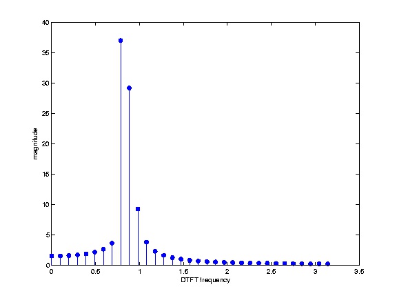
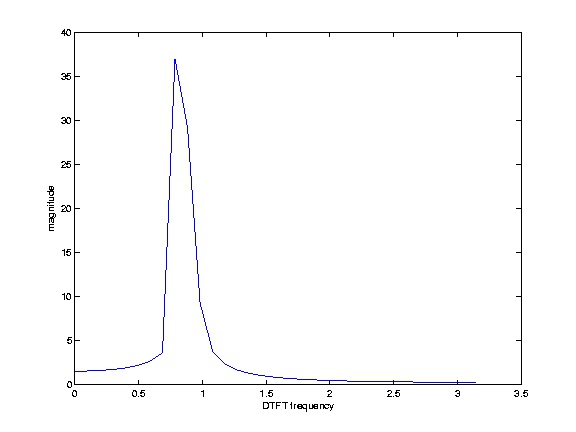
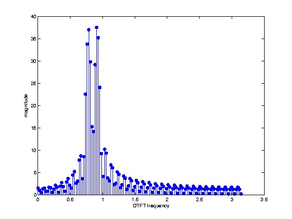
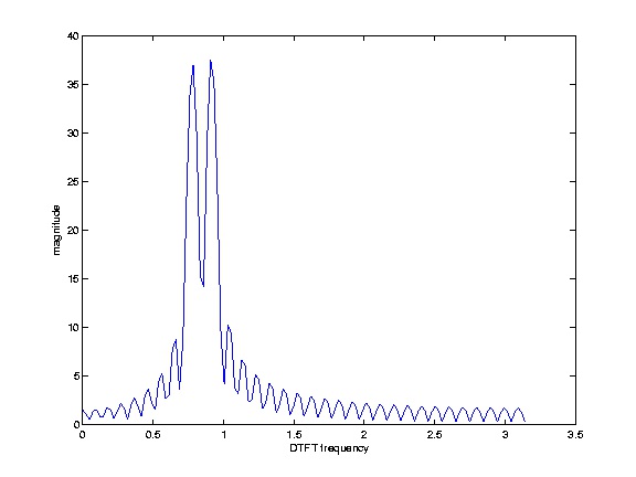
Figure 3.3 shows the magnitude of the DFT values corresponding to the non-negative frequencies
of a real-valued length-64 DFT of a length-64 signal, both in a "stem" format to emphasize the
discrete nature of the DFT frequency samples, and as a line plot to emphasize its use as an
approximation to the continuous-in-frequency DTFT. From this figure, it appears that the signal
has a single dominant frequency component.
<db:title>Stem plot</db:title>
(a)
<db:title>Line Plot</db:title>
(b)
Figure 3.3. Spectrum without zero-padding
Magnitude DFT spectrum of 64 samples of a signal with a length-64 DFT (no zero padding)
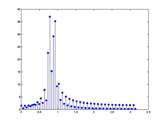
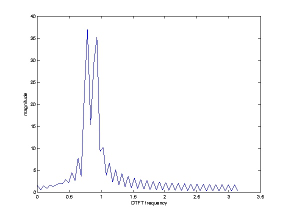
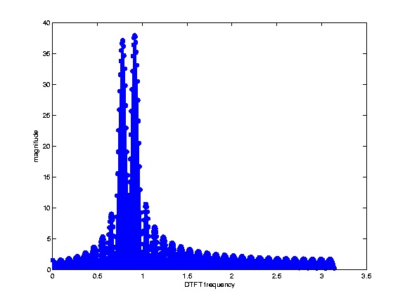
Zero-padding by a factor of two by appending 64 zero values to the signal and computing a length-
128 DFT yields Figure 3.4. It can now be seen that the signal consists of at least two narrowband
frequency components; the gap between them fell between DFT samples in Figure 3.3, resulting in
a misleading picture of the signal's spectral content. This is sometimes called the picket-fence
effect, and is a result of insufficient sampling in frequency. While zero-padding by a factor of two
has revealed more structure, it is unclear whether the peak magnitudes are reliably rendered, and
the jagged linear interpolation in the line graph does not yet reflect the smooth, continuously-
differentiable spectrum of the DTFT of a finite-length truncated signal. Errors in the apparent
peak magnitude due to insufficient frequency sampling is sometimes referred to as scalloping
loss.
<db:title>Stem plot</db:title>
(a)
<db:title>Line Plot</db:title>
(b)
Figure 3.4. Spectrum with factor-of-two zero-padding
Magnitude DFT spectrum of 64 samples of a signal with a length-128 DFT (double-length zero-padding)
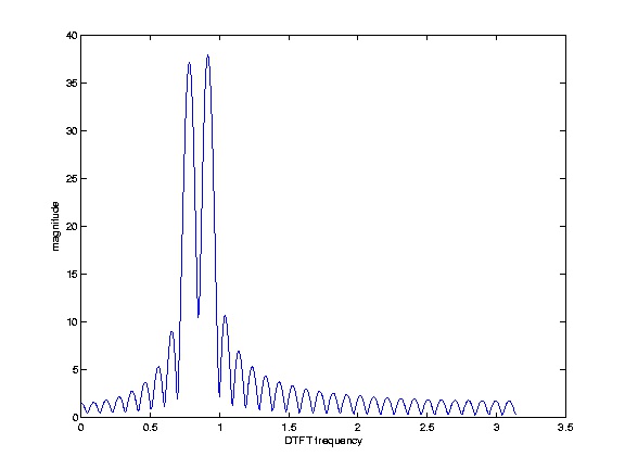
Zero-padding to four times the length of the signal, as shown in Figure 3.5, clearly shows the
spectral structure and reveals that the magnitude of the two spectral lines are nearly identical. The
line graph is still a bit rough and the peak magnitudes and frequencies may not be precisely
captured, but the spectral characteristics of the truncated signal are now clear.
<db:title>Stem plot</db:title>
(a)
<db:title>Line Plot</db:title>
(b)
Figure 3.5. Spectrum with factor-of-four zero-padding
Magnitude DFT spectrum of 64 samples of a signal with a length-256 zero-padded DFT (four times zero-padding)
Zero-padding to a length of 1024, as shown in Figure 3.6 yields a spectrum that is smooth and
continuous to the resolution of the computer screen, and produces a very accurate rendition of the
DTFT of the truncated signal.
<db:title>Stem plot</db:title>
(a)
<db:title>Line Plot</db:title>
(b)
Figure 3.6. Spectrum with factor-of-sixteen zero-padding
Magnitude DFT spectrum of 64 samples of a signal with a length-1024 zero-padded DFT. The spectrum now looks smooth and
continuous and reveals all the structure of the DTFT of a truncated signal.


The signal used in this example actually consisted of two pure sinusoids of equal magnitude. The
slight difference in magnitude of the two dominant peaks, the breadth of the peaks, and the sinc-
like lesser side lobe peaks throughout frequency are artifacts of the truncation, or windowing,
process used to practically approximate the DFT. These problems and partial solutions to them are
discussed in the following section.
Effects of Windowing
Applying the DTFT multiplication property
we find that the
DFT of the windowed (truncated) signal produces samples not of the true (desired) DTFT
spectrum X( ω) , but of a smoothed verson X( ω)* W( ω) . We want this to resemble X( ω) as closely as possible, so W( ω) should be as close to an impulse as possible. The window w( n) need not be a simple truncation (or rectangle, or boxcar) window; other shapes can also be used as long as
they limit the sequence to at most N consecutive nonzero samples. All good windows are impulse-
like, and represent various tradeoffs between three criteria:
1. main lobe width: (limits resolution of closely-spaced peaks of equal height)
2. height of first sidelobe: (limits ability to see a small peak near a big peak)
3. slope of sidelobe drop-off: (limits ability to see small peaks further away from a big peak)
Many different window functions have been developed for truncating and shaping a length- N
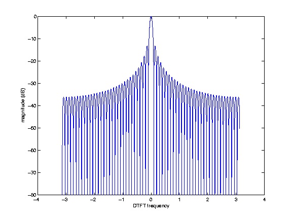
signal segment for spectral analysis. The simple truncation window has a periodic sinc DTFT, as
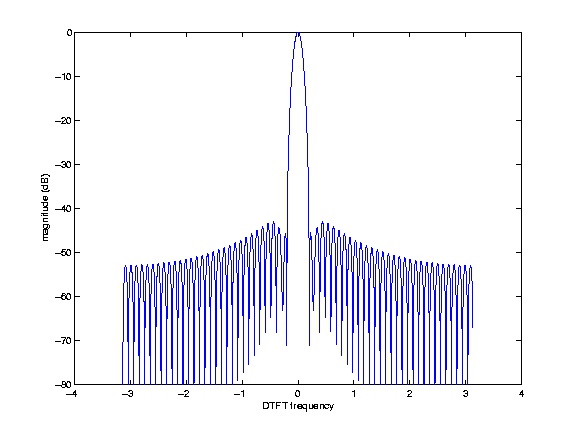
shown in Figure 3.7. It has the narrowest main-lobe width,
at the -3 dB level and
between
the two zeros surrounding the main lobe, of the common window functions, but also the largest
side-lobe peak, at about -13 dB. The side-lobes also taper off relatively slowly.
<db:title>Rectangular window</db:title>
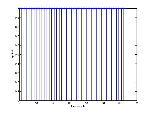
(a)
<db:title>Magnitude of boxcar window spectrum</db:title>
(b)
Figure 3.7.
Length-64 truncation (boxcar) window and its magnitude DFT spectrum


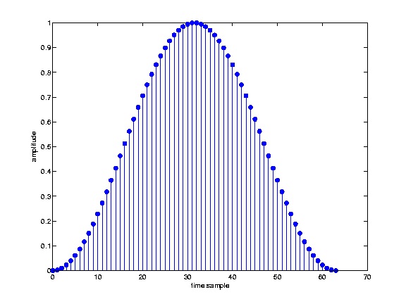
The Hann window (sometimes also called the hanning window), illustrated in Figure 3.8, takes the form
for n between 0 and N−1 . It has a main-lobe width (about
at the -
3 dB level and
between the two zeros surrounding the main lobe) considerably larger than the
rectangular window, but the largest side-lobe peak is much lower, at about -31.5 dB. The side-
lobes also taper off much faster. For a given length, this window is worse than the boxcar window
at separating closely-spaced spectral components of similar magnitude, but better for identifying
smaller-magnitude components at a greater distance from the larger components.
<db:title>Hann window</db:title>
(a)
<db:title>Magnitude of Hann window spectrum</db:title>
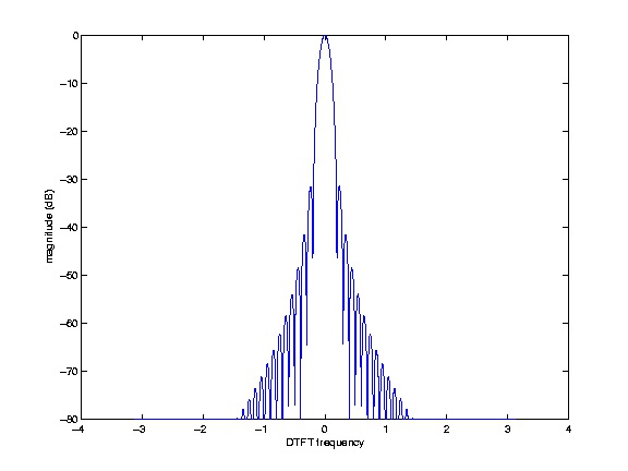


(b)
Figure 3.8.
Length-64 Hann window and its magnitude DFT spectrum
The Hamming window, illustrated in Figure 3.9, has a form similar to the Hann window but with slightly different constants:
for n between 0 and N−1 . Since it is composed
of the same Fourier series harmonics as the Hann window, it has a similar main-lobe width (a bit
less than
at the -3 dB level and
between the two zeros surrounding the main lobe), but the
largest side-lobe peak is much lower, at about -42.5 dB. However, the side-lobes also taper off
much more slowly than with the Hann window. For a given length, the Hamming window is better
than the Hann (and of course the boxcar) windows at separating a small component relatively near
to a large component, but worse than the Hann for identifying very small components at
considerable frequency separation. Due to their shape and form, the Hann and Hamming windows
are also known as raised-cosine windows.
<db:title>Hamming window</db:title>
(a)
<db:title>Magnitude of Hamming window spectrum</db:title>
(b)
Figure 3.9.
Length-64 Hamming window and its magnitude DFT spectrum


Standard even-length windows are symmetric around a point halfway between the window
samples
and . For some applications such as time-frequency analysis, it may be
important to align the window perfectly to a sample. In such cases, a DFT-symmetric window
that is symmetric around the -th sample can be used. For example, the DFT-symmetric
Hamming window is
. A DFT-symmetric window has a purely real-
valued DFT and DTFT. DFT-symmetric versions of windows, such as the Hamming and Hann
windows, composed of few discrete Fourier series terms of period N, have few non-zero DFT
terms (only when not zero-padded) and can be used efficiently in running FFTs.
The main-lobe width of a window is an inverse function of the window-length N ; for any type of
window, a longer window will always provide better resolution.
Many other windows exist that make various other tradeoffs between main-lobe width, height of
largest side-lobe, and side-lobe rolloff rate. The Kaiser window family, based on a modified Bessel function, has an adjustable parameter that allows the user to tune the tradeoff over a
continuous range. The Kaiser window has near-optimal time-frequency resolution and is widely
used. A list of many different windows can be found here.
Example 3.1.
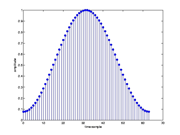
Figure 3.10 shows 64 samples of a real-valued signal composed of several sinusoids of various
frequencies and amplitudes.
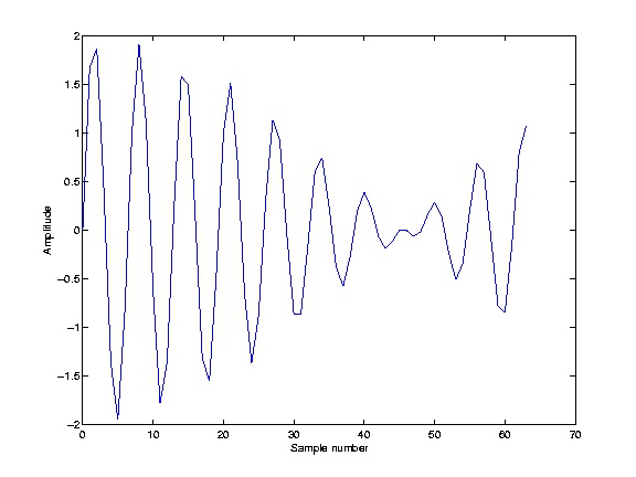
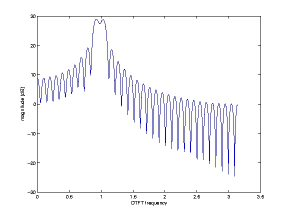
Figure 3.10.
64 samples of an unknown signal
Figure 3.11 shows the magnitude (in dB) of the positive frequencies of a length-1024 zero-
padded DFT of this signal (that is, using a simple truncation, or rectangular, window).
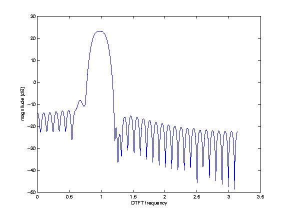
Figure 3.11.
Magnitude (in dB) of the zero-padded DFT spectrum of the signal in Figure 3.10 using a simple length-64 rectangular window From this spectrum, it is clear that the signal has two large, nearby frequency components
with frequencies near 1 radian of essentially the same magnitude.
Figure 3.12 shows the spectral estimate produced using a length-64 Hamming window applied
to the same signal shown in Figure 3.10.
Figure 3.12.
Magnitude (in dB) of the zero-padded DFT spectrum of the signal in Figure 3.10 using a length-64 Hamming window The two large spectral peaks can no longer be resolved; they blur into a single broad peak due
to the reduced spectral resolution of the broader main lobe of the Hamming window. However,
the lower side-lobes reveal a third component at a frequency of about 0.7 radians at about 35
dB lower magnitude than the larger components. This component was entirely buried under
the side-lobes when the rectangular window was used, but now stands out well above the much
lower nearby side-lobes of the Hamming window.
Figure 3.13 shows the spectral estimate produced using a length-64 Hann window applied to
the same signal shown in Figure 3.10.
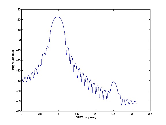
Figure 3.13.
Magnitude (in dB) of the zero-padded DFT spectrum of the signal in Figure 3.10 using a length-64 Hann window The two large components again merge into a single peak, and the smaller component
observed with the Hamming window is largely lost under the higher nearby side-lobes of the
Hann window. However, due to the much faster side-lobe rolloff of the Hann window's
spectrum, a fourth component at a frequency of about 2.5 radians with a magnitude about 65
dB below that of the main peaks is now clearly visible.
This example illustrates that no single window is best for all spectrum analyses. The best
window depends on the nature of the signal, and different windows may be better for different
components of the same signal. A skilled spectrum analysist may apply several different
windows to a signal to gain a fuller understanding of the data.
Classical Statistical Spectral Estimation*
Many signals are either partly or wholly stochastic, or random. Important examples include
human speech, vibration in machines, and CDMA communication signals. Given the ever-present noise in electronic systems, it can be argued that almost all signals are at least partly stochastic.
Such signals may have a distinct average spectral structure that reveals important information
(such as for speech recognition or early detection of damage in machinery). Spectrum analysis of
any single block of data using window-based deterministic spectrum analysis, however,
produces a random spectrum that may be difficult to interpret. For such situations, the classical


statistical spectrum estimation methods described in this module can be used.
The goal in classical statistical spectrum analysis is to estimate E[(| X( ω)|)2] , the power spectral
density (PSD) across frequency of the stochastic signal. That is, the goal is to find the expected
(mean, or average) energy density of the signal as a function of frequency. (For zero-mean signals,
this equals the variance of each frequency sample.) Since the spectrum of each block of signal
samples is itself random, we must average the squared spectral magnitudes over a number of
blocks of data to find the mean. There are two main classical approaches, the periodogram and
auto-correlation methods.