

3. Post multiply by to get
to get X( zk) .
1. and 3. require N and M operations respectively. 2. can be performed efficiently using fast convolution.
Figure 3.49.
is required only for –(( N−1))≤ n≤ M−1 , so this linear convolution can be implemented with
L≥ N+ M−1 FFTs.
Wrap
around L when implementing with circular convolution.
So, a weird-length DFT can be implemented relatively efficiently using power-of-two algorithms via the chirp-z transform.
Also useful for "zoom-FFTs".
3.6. FFTs of prime length and Rader's conversion*
The power-of-two FFT algorithms, such as the radix-2 and radix-4 FFTs, and the common-
factor and prime-factor FFTs, achieve great reductions in computational complexity of the DFT
when the length, N, is a composite number. DFTs of prime length are sometimes needed, however,
particularly for the short-length DFTs in common-factor or prime-factor algorithms. The methods
described here, along with the composite-length algorithms, allow fast computation of DFTs of
any length.
There are two main ways of performing DFTs of prime length:
1. Rader's conversion, which is most efficient, and the
2. Chirp-z transform, which is simpler and more general.
Oddly enough, both work by turning prime-length DFTs into convolution! The resulting
convolutions can then be computed efficiently by either
1. fast convolution via composite-length FFTs (simpler) or by
2. Winograd techniques (more efficient)
Rader's Conversion
Rader's conversion is a one-dimensional index-mapping scheme that turns a length- N DFT ( N
prime) into a length-( N−1 ) convolution and a few additions. Rader's conversion works only for
prime-length N.
An index map simply rearranges the order of the sum operation in the DFT definition. Because addition is a commutative operation, the same mathematical result is produced from any order, as
long as all of the same terms are added once and only once. (This is the condition that defines an
index map.) Unlike the multi-dimensional index maps used in deriving common factor and
prime-factor FFTs, Rader's conversion uses a one-dimensional index map in a finite group of N
integers: k=( rm)mod N
Fact from number theory
If N is prime, there exists an integer " r" called a primitive root, such that the index map
k=( rm)mod N , m=[0, 1, 2, …, N−2] , uniquely generates all elements k=[1, 2, 3, …, N−1]
Example 3.5.
N=5 , r=2 (20)mod5=1 (21)mod5=2 (22)mod5=4 (23)mod5=3
Another fact from number theory
For N prime, the inverse of r (i.e. ( r-1 r)mod N=1 is also a primitive root (call it r-1 ).
Example 3.6.


N=5 , r=2 r-1=3 (2×3)mod5=1 (30)mod5=1 (31)mod5=3 (32)mod5=4 (33)mod5=2
So why do we care? Because we can use these facts to turn a DFT into a convolution!
Rader's Conversion
Let n=( r– m)mod N , m=[0, 1, …, N−2]∧ n∈[1, 2, …, N−1] , k=( rp)mod N , p=[0, 1, …, N−2]∧ k∈[1, 2, …, N−1]
where for convenience
in the DFT equation. For k≠0
()
where l=[0, 1, …, N−2]
Example 3.7.
N=5 , r=2 , r-1=3
where for visibility the matrix
entries represent only the power, m of the corresponding DFT term W m
N Note that the 4-by-4
corresponds to a length-4 circular convolution.
Rader's conversion turns a prime-length DFT into a few adds and a composite-length ( N−1 ) circular convolution, which can be computed efficiently using either
1. fast convolution via FFT and IFFT
2. index-mapped convolution algorithms and short Winograd convolution alogrithms. (Rather
complicated, and trades fewer multiplies for many more adds, which may not be worthwile on
most modern processors.) See R.C. Agarwal and J.W. Cooley [link]
Winograd minimum-multiply convolution and DFT algorithms


S. Winograd has proved that a length- N circular or linear convolution or DFT requires less than 2 N multiplies (for real data), or 4 N real multiplies for complex data. (This doesn't count
multiplies by rational fractions, like 3 or or , which can be computed with additions and one
overall scaling factor.) Furthermore, Winograd showed how to construct algorithms achieving
these counts. Winograd prime-length DFTs and convolutions have the following characteristics:
1. Extremely efficient for small N ( N<20 )
2. The number of adds becomes huge for large N.
Thus Winograd's minimum-multiply FFT's are useful only for small N. They are very important
for Prime-Factor Algorithms, which generally use Winograd modules to implement the short-length DFTs. Tables giving the multiplies and adds necessary to compute Winograd FFTs for
various lengths can be found in C.S. Burrus (1988) [link]. Tables and FORTRAN and TMS32010
programs for these short-length transforms can be found in C.S. Burrus and T.W. Parks (1985)
[link]. The theory and derivation of these algorithms is quite elegant but requires substantial background in number theory and abstract algebra. Fortunately for the practitioner, all of the short
algorithms one is likely to need have already been derived and can simply be looked up without
mastering the details of their derivation.
Winograd Fourier Transform Algorithm (WFTA)
The Winograd Fourier Transform Algorithm (WFTA) is a technique that recombines the short
Winograd modules in a prime-factor FFT into a composite- N structure with fewer multiplies but more adds. While theoretically interesting, WFTAs are complicated and different for every length,
and on modern processors with hardware multipliers the trade of multiplies for many more adds is
very rarely useful in practice today.
References
1. R.C. Agarwal and J.W. Cooley. (1977, Oct). New Algorithms for Digital Convolution. IEEE
Trans. on Acoustics, Speech, and Signal Processing, 25, 392-410.
2. C.S. Burrus. (1988). Efficient Fourier Transform and Convolution Algorithms. In J.S. Lin and
A.V. Oppenheim (Eds.), Advanced Topics in Signal Processing. Prentice-Hall.
3. C.S. Burrus and T.W. Parks. (1985). DFT/FFT and Convolution Algorithms. Wiley-
Interscience.
3.7. Choosing the Best FFT Algorithm*
3.7. Choosing the Best FFT Algorithm*
Choosing an FFT length
The most commonly used FFT algorithms by far are the power-of-two-length FFT algorithms.
The Prime Factor Algorithm (PFA) and Winograd Fourier Transform Algorithm (WFTA)
require somewhat fewer multiplies, but the overall difference usually isn't sufficient to warrant
the extra difficulty. This is particularly true now that most processors have single-cycle pipelined
hardware multipliers, so the total operation count is more relevant. As can be seen from the
following table, for similar lengths the split-radix algorithm is comparable in total operations to
the Prime Factor Algorithm, and is considerably better than the WFTA, although the PFA and
WTFA require fewer multiplications and more additions. Many processors now support single
cycle multiply-accumulate (MAC) operations; in the power-of-two algorithms all multiplies can
be combined with adds in MACs, so the number of additions is the most relevant indicator of
computational cost.
Table 3.4. Representative FFT Operation Counts
FFT length Multiplies (real) Adds(real) Mults + Adds
Radix 2
1024
10248
30728
40976
Split Radix
1024
7172
27652
34824
Prime Factor Alg 1008
5804
29100
34904
Winograd FT Alg 1008
3548
34416
37964
The Winograd Fourier Transform Algorithm is particularly difficult to program and is rarely
used in practice. For applications in which the transform length is somewhat arbitrary (such as
fast convolution or general spectrum analysis), the length is usually chosen to be a power of two.
When a particular length is required (for example, in the USA each carrier has exactly 416
frequency channels in each band in the AMPS cellular telephone standard), a Prime Factor
Algorithm for all the relatively prime terms is preferred, with a Common Factor Algorithm for other non-prime lengths. Winograd's short-length modules should be used for the prime-length factors that are not powers of two. The chirp z-transform offers a universal way to compute any length DFT (for example, Matlab reportedly uses this method for lengths other than a power of two), at a few times higher cost than that of a CFA or PFA optimized for that specific length. The
chirp z-transform, along with Rader's conversion, assure us that algorithms of O( NlogN) complexity exist for any DFT length N .
Selecting a power-of-two-length algorithm
The choice of a power-of-two algorithm may not just depend on computational complexity. The
latest extensions of the split-radix algorithm offer the lowest known power-of-two FFT operation counts, but the 10%-30% difference may not make up for other factors such as regularity of
structure or data flow, FFT programming tricks, or special hardware features. For example, the
decimation-in-time radix-2 FFT is the fastest FFT on Texas Instruments' TMS320C54x DSP
microprocessors, because this processor family has special assembly-language instructions that
accelerate this particular algorithm. On other hardware, radix-4 algorithms may be more
efficient. Some devices, such as AMI Semiconductor's Toccata ultra-low-power DSP
microprocessor family, have on-chip FFT accelerators; it is always faster and more power-
efficient to use these accelerators and whatever radix they prefer. For fast convolution, the
decimation-in-frequency algorithms may be preferred because the bit-reversing can be bypassed; however, most DSP microprocessors provide zero-overhead bit-reversed indexing hardware and
prefer decimation-in-time algorithms, so this may not be true for such machines. Good, compiler-
or hardware-friendly programming always matters more than modest differences in raw operation
counts, so manufacturers' or good third-party FFT libraries are often the best choice. The module
FFT programming tricks references some good, free FFT software (including the FFTW
package) that is carefully coded to be compiler-friendly; such codes are likely to be considerably
faster than codes written by the casual programmer.
Multi-dimensional FFTs
Multi-dimensional FFTs pose additional possibilities and problems. The orthogonality and
separability of multi-dimensional DFTs allows them to be efficiently computed by a series of one-
dimensional FFTs along each dimension. (For example, a two-dimensional DFT can quickly be
computed by performing FFTs of each row of the data matrix followed by FFTs of all columns, or
vice-versa.) Vector-radix FFTs have been developed with higher efficiency per sample than row-
column algorithms. Multi-dimensional datasets, however, are often large and frequently exceed
the cache size of the processor, and excessive cache misses may increase the computational time
greatly, thus overwhelming any minor complexity reduction from a vector-radix algorithm. Either
vector-radix FFTs must be carefully programmed to match the cache limitations of a specific
processor, or a row-column approach should be used with matrix transposition in between to
ensure data locality for high cache utilization throughout the computation.
Few time or frequency samples
FFT algorithms gain their efficiency through intermediate computations that can be reused to
compute many DFT frequency samples at once. Some applications require only a handful of
frequency samples to be computed; when that number is of order less than O( logN) , direct
computation of those values via Goertzel's algorithm is faster. This has the additional advantage that any frequency, not just the equally-spaced DFT frequency samples, can be selected. Sorensen
and Burrus [link] developed algorithms for when most input samples are zero or only a block of DFT frequencies are needed, but the computational cost is of the same order.
Some applications, such as time-frequency analysis via the short-time Fourier transform or
spectrogram, require DFTs of overlapped blocks of discrete-time samples. When the step-size
between blocks is less than O( logN) , the running FFT will be most efficient. (Note that any
window must be applied via frequency-domain convolution, which is quite efficient for sinusoidal windows such as the Hamming window. ) For step-sizes of O( logN) or greater, computation of the DFT of each successive block via an FFT is faster.
References
1. H.V. Sorensen and C.S. Burrus. (1993). Efficient computation of the DFT with only a subset of
input or output points. IEEE Transactions on Signal Processing, 41(3), 1184-1200.
Solutions


Chapter 4. Wavelets
4.1. Time Frequency Analysis and Continuous Wavelet
Transform
Why Transforms? *
In the field of signal processing we frequently encounter the use of transforms. Transforms are
named such because they take a signal and transform it into another signal, hopefully one which
is easier to process or analyze than the original. Essentially, transforms are used to manipulate
signals such that their most important characteristics are made plainly evident. To isolate a
signal's important characteristics, however, one must employ a transform that is well matched to
that signal. For example, the Fourier transform, while well matched to certain classes of signal,
does not efficiently extract information about signals in other classes. This latter fact motivates
our development of the wavelet transform.
Limitations of Fourier Analysis*
Let's consider the Continuous-Time Fourier Transform (CTFT) pair:
The Fourier transform pair supplies us with our notion of "frequency." In other
words, all of our intuitions regarding the relationship between the time domain and the frequency
domain can be traced to this particular transform pair.
It will be useful to view the CTFT in terms of basis elements. The inverse CTFT equation above
says that the time-domain signal x( t) can be expressed as a weighted summation of basis
elements , where bΩ( t)= ⅇⅈΩt is the basis element corresponding to frequency Ω. In other words, the basis elements are parameterized by the variable Ω that we call frequency. Finally,
X( Ω) specifies the weighting coefficient for bΩ( t) . In the case of the CTFT, the number of basis elements is uncountably infinite, and thus we need an integral to express the summation.
The Fourier Series (FS) can be considered as a special sub-case of the CTFT that applies when the
time-domain signal is periodic. Recall that if x( t) is periodic with period T, then it can be
expressed as a weighted summation of basis elements
, where
:


Here the basis elements comes from a countably-infinite set, parameterized
by the frequency index k∈ℤ . The coefficients
specify the strength of the corresponding
basis elements within signal x( t) .
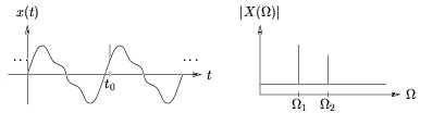
Though quite popular, Fourier analysis is not always the best tool to analyze a signal whose
characteristics vary with time. For example, consider a signal composed of a periodic component
plus a sharp "glitch" at time t 0 , illustrated in time- and frequency-domains, Figure 4.1.
Figure 4.1.
Fourier analysis is successful in reducing the complicated-looking periodic component into a few
simple parameters: the frequencies and their corresponding magnitudes/phases. The glitch
component, described compactly in terms of the time-domain location t 0 and amplitude, however,
is not described efficiently in the frequency domain since it produces a wide spread of frequency
components. Thus, neither time- nor frequency-domain representations alone give an efficient
description of the glitched periodic signal: each representation distills only certain aspects of the
signal.
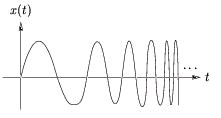
As another example, consider the linear chirp x( t)=sin( Ωt 2) illustrated in Figure 4.2.
Figure 4.2.
Though written using the sin( ·) function, the chirp is not described by a single Fourier frequency.
We might try to be clever and write sin( Ωt 2)=sin( Ωt·t)=sin( Ω( t) ·t) where it now seems that signal has an instantaneous frequency Ω( t)= Ωt which grows linearly in time. But here we must be
cautious! Our newly-defined instantaneous frequency Ω( t) is not consistent with the Fourier
notion of frequency. Recall that