multiplications, or fewer real multiplies than other ones. By implementing special butterflies for
these twiddle factors as discussed in FFT algorithm and programming tricks, the computational cost of the radix-2 decimation-in-frequency FFT can be reduced to
2 N log2 N−7 N+12 real multiplies
3 N log2 N−3 N+4 real additions
The decimation-in-frequency FFT is a flow-graph reversal of the decimation-in-time FFT: it has the same twiddle factors (in reverse pattern) and the same operation counts.
In a decimation-in-frequency radix-2 FFT as illustrated in Figure 3.32, the output is in bit-
reversed order (hence "decimation-in-frequency"). That is, if the frequency-sample index n is
written as a binary number, the order is that binary number reversed. The bit-reversal process
is illustrated here.
It is important to note that, if the input data are in order before beginning the FFT computations,
the outputs of each butterfly throughout the computation can be placed in the same memory
locations from which the inputs were fetched, resulting in an in-place algorithm that requires no
extra memory to perform the FFT. Most FFT implementations are in-place, and overwrite the
input data with the intermediate values and finally the output.
Alternate FFT Structures*
Bit-reversing the input in decimation-in-time (DIT) FFTs or the output in decimation-in-
frequency (DIF) FFTs can sometimes be inconvenient or inefficient. For such situations,
alternate FFT structures have been developed. Such structures involve the same mathematical
computations as the standard algorithms, but alter the memory locations in which intermediate
values are stored or the order of computation of the FFT butterflies.
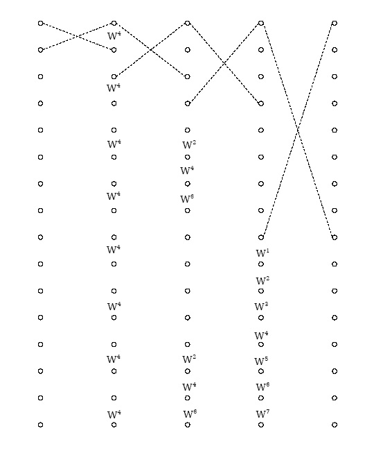
The structure in Figure 3.33 computes a decimation-in-frequency FFT, but remaps the memory usage so that the input is bit-reversed, and the output is in-order as in the conventional
decimation-in-time FFT. This alternate structure is still considered a DIF FFT because the
twiddle factors are applied as in the DIF FFT. This structure is useful if for some reason the DIF
butterfly is preferred but it is easier to bit-reverse the input.
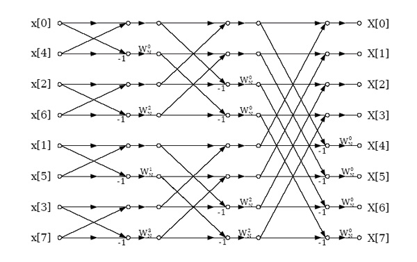
Figure 3.33.
Decimation-in-frequency radix-2 FFT with bit-reversed input. This is an in-place algorithm in which the same memory can be reused throughout the computation.
There is a similar structure for the decimation-in-time FFT with in-order inputs and bit-reversed frequencies. This structure can be useful for fast convolution on machines that favor decimation-in-time algorithms because the filter can be stored in bit-reverse order, and then the inverse FFT
returns an in-order result without ever bit-reversing any data. As discussed in Efficient FFT
Programming Tricks, this may save several percent of the execution time.
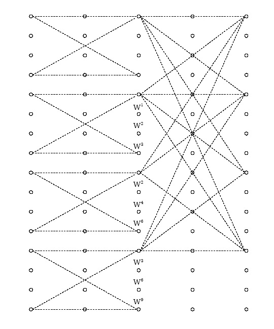
The structure in Figure 3.34 implements a decimation-in-frequency FFT that has both input and output in order. It thus avoids the need for bit-reversing altogether. Unfortunately, it destroys the
in-place structure somewhat, making an FFT program more complicated and requiring more
memory; on most machines the resulting cost exceeds the benefits. This structure can be
computed in place if two butterflies are computed simultaneously.
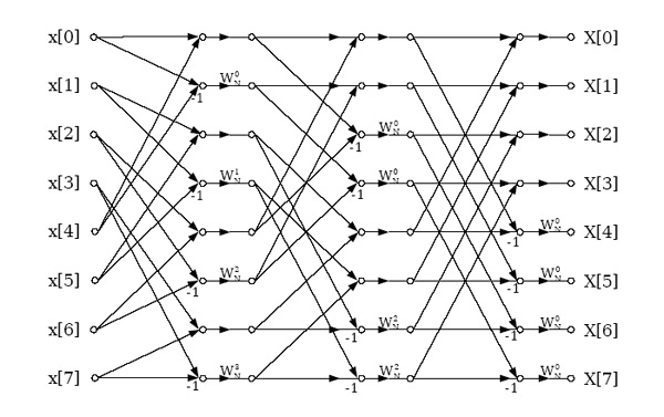
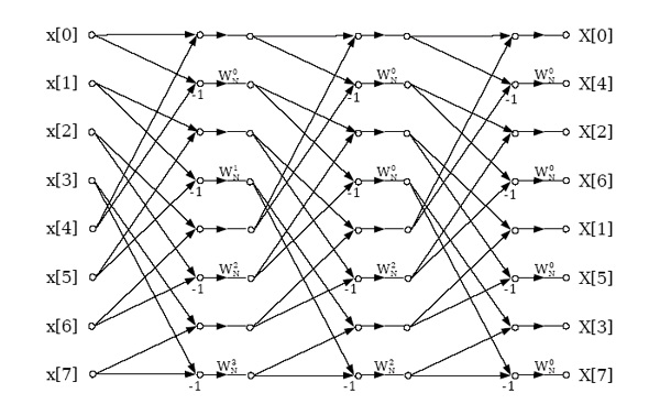
Figure 3.34.
Decimation-in-frequency radix-2 FFT with in-order input and output. It can be computed in-place if two butterflies are computed
simultaneously.
The structure in Figure 3.35 has a constant geometry; the connections between memory locations
are identical in each FFT stage. Since it is not in-place and requires bit-reversal, it is inconvenient for software implementation, but can be attractive for a highly parallel hardware implementation
because the connections between stages can be hardwired. An analogous structure exists that has
bit-reversed inputs and in-order outputs.
Figure 3.35.


This constant-geometry structure has the same interconnect pattern from stage to stage. This structure is sometimes useful for special hardware.
Radix-4 FFT Algorithms*
The radix-4 decimation-in-time and decimation-in-frequency fast Fourier transforms (FFTs)
gain their speed by reusing the results of smaller, intermediate computations to compute multiple
DFT frequency outputs. The radix-4 decimation-in-time algorithm rearranges the discrete
Fourier transform (DFT) equation into four parts: sums over all groups of every fourth discrete-time index n=[0, 4, 8, …, N−4] , n=[1, 5, 9, …, N−3] , n=[2, 6, 10, …, N−2] and n=[3, 7, 11, …, N−1] as in Equation. (This works out only when the FFT length is a multiple of four.) Just as in the radix-2 decimation-in-time FFT, further mathematical manipulation shows that the length- N DFT can be computed as the sum of the outputs of four length- DFTs, of the
even-indexed and odd-indexed discrete-time samples, respectively, where three of them are
multiplied by so-called twiddle factors
,
, and
.
()
This is called a decimation in time because the time samples are rearranged in alternating groups,
and a radix-4 algorithm because there are four groups. Figure 3.36 graphically illustrates this form of the DFT computation.


Figure 3.36. Radix-4 DIT structure
Decimation in time of a length- N DFT into four length-
DFTs followed by a combining stage.
Due to the periodicity with of the short-length DFTs, their outputs for frequency-sample k are
reused to compute X( k) ,
,
, and
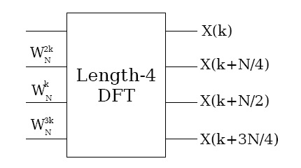
. It is this reuse that gives the radix-4 FFT its
efficiency. The computations involved with each group of four frequency samples constitute the
radix-4 butterfly, which is shown in Figure 3.37. Through further rearrangement, it can be shown that this computation can be simplified to three twiddle-factor multiplies and a length-4 DFT! The
theory of multi-dimensional index maps shows that this must be the case, and that FFTs of any factorable length may consist of successive stages of shorter-length FFTs with twiddle-factor
multiplications in between. The length-4 DFT requires no multiplies and only eight complex
additions (this efficient computation can be derived using a radix-2 FFT).


(a)
(b)
Figure 3.37.
The radix-4 DIT butterfly can be simplified to a length-4 DFT preceded by three twiddle-factor multiplies.
If the FFT length N=4 M , the shorter-length DFTs can be further decomposed recursively in the
same manner to produce the full radix-4 decimation-in-time FFT. As in the radix-2 decimation-
in-time FFT, each stage of decomposition creates additional savings in computation. To
determine the total computational cost of the radix-4 FFT, note that there are
stages, each with butterflies per stage. Each radix-4 butterfly requires 3 complex multiplies and
8 complex additions. The total cost is then
Radix-4 FFT Operation Counts
complex multiplies (75% of a radix-2 FFT)
complex adds (same as a radix-2 FFT)
The radix-4 FFT requires only 75% as many complex multiplies as the radix-2 FFTs, although it uses the same number of complex additions. These additional savings make it a widely-used FFT
algorithm.
The decimation-in-time operation regroups the input samples at each successive stage of
decomposition, resulting in a "digit-reversed" input order. That is, if the time-sample index n is
written as a base-4 number, the order is that base-4 number reversed. The digit-reversal process is
illustrated for a length- N=64 example below.
Example 3.4. N = 64 = 4^3
Table 3.2.
Original
Original Digit
Reversed Digit
Digit-Reversed
Number
Order
Order
Number
0
000
000
0
1
001
100
16
2
002
200
32
3
003
300
48
4
010
010
4
5
011
110
20
⋮
⋮
⋮
⋮
It is important to note that, if the input signal data are placed in digit-reversed order before
beginning the FFT computations, the outputs of each butterfly throughout the computation can be
placed in the same memory locations from which the inputs were fetched, resulting in an in-place
algorithm that requires no extra memory to perform the FFT. Most FFT implementations are in-
place, and overwrite the input data with the intermediate values and finally the output. A slight
rearrangement within the radix-4 FFT introduced by Burrus [link] allows the inputs to be arranged in bit-reversed rather than digit-reversed order.
A radix-4 decimation-in-frequency FFT can be derived similarly to the radix-2 DIF FFT, by separately computing all four groups of every fourth output frequency sample. The DIF radix-4
FFT is a flow-graph reversal of the DIT radix-4 FFT, with the same operation counts and twiddle
factors in the reversed order. The output ends up in digit-reversed order for an in-place DIF
algorithm.
How do we derive a radix-4 algorithm when N=4 M 2 ?
Perform a radix-2 decomposition for one stage, then radix-4 decompositions of all subsequent
shorter-length DFTs.
References
1. C.S. Burrus. (1988, July). Unscrambling for fast DFT algorithms. IEEE Transactions on
Acoustics, Speech, and Signal Processing, ASSP-36(7), 1086-1089.
Split-radix FFT Algorithms*
The split-radix algorithm, first clearly described and named by Duhamel and Hollman [link] in 1984, required fewer total multiply and add operations operations than any previous power-of-two
algorithm. ( Yavne [link] first derived essentially the same algorithm in 1968, but the description was so atypical that the work was largely neglected.) For a time many FFT experts thought it to be
optimal in terms of total complexity, but even more efficient variations have more recently been
discovered by Johnson and Frigo [link].
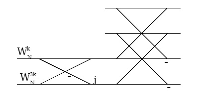
The split-radix algorithm can be derived by careful examination of the radix-2 and radix-4
flowgraphs as in Figure 1 below. While in most places the radix-4 algorithm has fewer nontrivial twiddle factors, in some places the radix-2 actually lacks twiddle factors present in the radix-4
structure or those twiddle factors simplify to multiplication by – ⅈ , which actually requires only
additions. By mixing radix-2 and radix-4 computations appropriately, an algorithm of lower complexity than either can be derived.
<db:title>radix-2</db:title>
<db:title>radix-4</db:title>
(b)
(a)
Figure 3.38. Motivation for split-radix algorithm
See Decimation-in-Time (DIT) Radix-2 FFT and Radix-4 FFT Algorithms for more information on these algorithms.
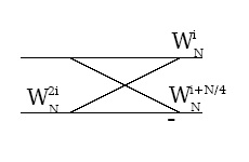
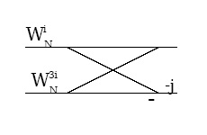
An alternative derivation notes that radix-2 butterflies of the form shown in Figure 2 can merge
twiddle factors from two successive stages to eliminate one-third of them; hence, the split-radix
algorithm requires only about two-thirds as many multiplications as a radix-2 FFT.

(a)
(b)
Figure 3.39.
Note that these two butterflies are equivalent
The split-radix algorithm can also be derived by mixing the radix-2 and radix-4 decompositions.
(3.3)
DIT Split-radix derivation
Figure 3 illustrates the resulting split-radix butterfly.
Figure 3.40. Decimation-in-Time Split-Radix Butterfly
The split-radix butterfly mixes radix-2 and radix-4 decompositions and is L-shaped
Further decomposition of the half- and quarter-length DFTs yields the full split-radix algorithm.
The mix of different-length FFTs in different parts of the flowgraph results in a somewhat
irregular algorithm; Sorensen et al. [link] show how to adjust the computation such that the data retains the simpler radix-2 bit-reverse order. A decimation-in-frequency split-radix FFT can be
derived analogously.
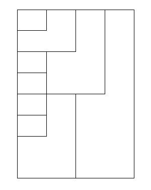


Figure 3.41.
The split-radix transform has L-shaped butterflies
The multiplicative complexity of the split-radix algorithm is only about two-thirds that of the
radix-2 FFT, and is better than the radix-4 FFT or any higher power-of-two radix as well. The
additions within the complex twiddle-factor multiplies are similarly reduced, but since the
underlying butterfly tree remains the same in all power-of-two algorithms, the butterfly additions
remain the same and the overall reduction in additions is much less.
Table 3.3. Operation Counts
Complex M/As Real M/As (4/2)
Real M/As (3/3)
Multiplies
N log2 N−3 N+4
Additions O[ N log2 N]
3 N log2 N−3 N+4
Comments
The split-radix algorithm has a somewhat irregular structure. Successful progams have been
written ( Sorensen [link]) for uni-processor machines, but it may be difficult to efficiently code the split-radix algorithm for vector or multi-processor machines.
G. Bruun's algorithm [link] requires only N−2 more operations than the split-radix algorithm and has a regular structure, so it might be better for multi-processor or special-purpose
hardware.
The execution time of FFT programs generally depends more on compiler- or hardware-


The execution time of FFT programs generally depends more on compiler- or hardware-
friendly software design than on the exact computational complexity. See Efficient FFT
Algorithm and Programming Tricks for further pointers and links to good code.
References
1. P. Duhamel and H. Hollman. (1984, Jan 5). Split-radix FFT algorithms. Electronics Letters,
20, 14-16.
2. R. Yavne. (1968). An economical method for calculating the discrete Fourier transform. Proc.
AFIPS Fall Joint Computer Conf., , 33, 115-125.
3. S.G Johnson and M. Frigo. (2006). A modified split-radix FFT with fewer arithmetic
operations. IEEE Transactions on Signal Processing, 54,
4. H.V. Sorensen, M.T. Heideman, and C.S. Burrus. (1986). On computing the split-radix FFT.
IEEE Transactions on Signal Processing, 34(1), 152-156.
5. G. Bruun. (1978, February). Z-Transform DFT Filters and FFTs. IEEE Transactions on Signal
Processing, 26, 56-63.
Efficient FFT Algorithm and Programming Tricks*
The use of FFT algorithms such as the radix-2 decimation-in-time or decimation-in-frequency
methods result in tremendous savings in computations when computing the discrete Fourier
transform. While most of the speed-up of FFTs comes from this, careful implementation can
provide additional savings ranging from a few percent to several-fold increases in program speed.
Precompute twiddle factors
, terms that multiply the intermediate data in the FFT
algorithms consist of cosines and sines that each take the equivalent of several multiplies to compute. However, at most N unique twiddle factors can appear in any FFT or DFT algorithm.
(For example, in the radix-2 decimation-in-time FFT, only twiddle factors
are used.) These twiddle factors can be precomputed once and stored in an
array in computer memory, and accessed in the FFT algorithm by table lookup. This simple
technique yields very substantial savings and is almost always used in practice.
Compiler-friendly programming
On most computers, only some of the total computation time of an FFT is spent performing the
FFT butterfly computations; determining indices, loading and storing data, computing loop
parameters and other operations consume the majority of cycles. Careful programming that allows
the compiler to generate efficient code can make a several-fold improvement in the run-time of an
FFT. The best choice of radix in terms of program speed may depend more on characteristics of
the hardware (such as the number of CPU registers) or compiler than on the exact number of
computations. Very often the manufacturer's library codes are carefully crafted by experts who
know intimately both the hardware and compiler architecture and how to get the most
performance out of them, so use of well-written FFT libraries is generally recommended. Certain
freely available programs and libraries are also very good. Perhaps the best current general-
purpose library is the FFTW package; information can be found at http://www.fftw.org. A paper by Frigo and Johnson [link] describes many of the key issues in developing compiler-friendly code.
Program in assembly la