Figure 4.21.
Using the fact that
is an orthonormal basis for W 1 , in conjunction with the wavelet
scaling equation,
()
where δ[ t− ℓ−2 n]=< φ( t− m), φ( t− ℓ−2 n)> .
The previous expression (Equation) indicates that { d 1[ n]} results from convolving { c 0[ m]} with a time-reversed version of g[ m] then downsampling by factor two (Figure 4.22).
Figure 4.22.
Putting these two operations together, we arrive at what looks like the analysis portion of an FIR
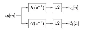


filterbank (Figure 4.23):
Figure 4.23.
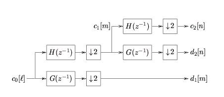
We can repeat this process at the next higher level. Since V 1=( W 2⊕ V 2) , there exist coefficients
{ c 2[ n]} and { d 2[ n]} such that
()
Using the same steps as before we find that
()
()
which gives a cascaded analysis filterbank (Figure 4.24):
Figure 4.24.
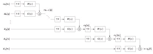
If we use V 0=( W 1⊕ W 2⊕ W 3⊕⋯⊕ Wk⊕ Vk) to repeat this process up to the k th level, we get the iterated analysis filterbank (Figure 4.25).
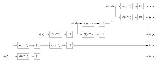

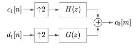

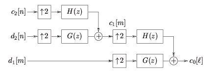
Figure 4.25.
As we might expect, signal reconstruction can be accomplished using cascaded two-channel
synthesis filterbanks. Using the same assumptions as before, we have:
()
where h[ m−2 n]=< φ 1 , n ( t), φ 0 , m ( t)> and g[ m−2 n]=< ψ 1 , n ( t), φ 0 , m ( t)> which can be implemented using the block diagram in Figure 4.26.
Figure 4.26.
The same procedure can be used to derive
()
from which we get the diagram in Figure 4.27.
Figure 4.27.
To reconstruct from the k th level, we can use the iterated synthesis filterbank (Figure 4.28).
Figure 4.28.
The table makes a direct comparison between wavelets and the two-channel orthogonal PR-FIR
filterbanks.
Table 4.3.
2-Channel Orthogonal PR-FIR
Discrete Wavelet Transform
Filterbank
Analysis-LPF
H( z-1)
H 0( z)
Power
H( z) H( z-1)+ H(– z) H(–( z-1))=2
H
Symmetry
0( z) H 0( z-1)+ H 0(– z) H 0(–( z-1))=1
Analysis HPF
G( z-1)
H 1( z)
Spectral
G( z)=±( z– PH(–( z-1))) , P is odd H
Reverse
1( z)=±( z–(( N−1)) H 0(–( z-1))) , N is even
Synthesis LPF H( z)
G 0( z)=2 z–(( N−1)) H 0( z-1)
Synthesis HPF G( z)
G 1( z)=2 z–(( N−1)) H 1( z-1)
From the table, we see that the discrete wavelet transform that we have been developing is
identical to two-channel orthogonal PR-FIR filterbanks in all but a couple details.
1. Orthogonal PR-FIR filterbanks employ synthesis filters with twice the gain of the analysis
filters, whereas in the DWT the gains are equal.
2. Orthogonal PR-FIR filterbanks employ causal filters of length N, whereas the DWT filters are
not constrained to be causal.


For convenience, however, the wavelet filters H( z) and G( z) are usually chosen to be causal. For
both to have even impulse response length N, we require that P= N−1 .
Initialization of the Wavelet Transform*
The filterbanks developed in the module on the filterbanks interpretation of the DWT start with the signal representation
and break the representation down into wavelet coefficients
and scaling coefficients at lower resolutions ( i.e. , higher levels k). The question remains: how do
we get the initial coefficients { c 0[ n]} ?
From their definition, we see that the scaling coefficients can be written using a convolution:
()
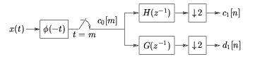
which suggests that the proper initialization of wavelet transform is accomplished by passing the
continuous-time input x( t) through an analog filter with impulse response φ(– t) and sampling its
output at integer times (Figure 4.29).
Figure 4.29.
Practically speaking, however, it is very difficult to build an analog filter with impulse response
φ(– t) for typical choices of scaling function.
The most often-used approximation is to set c 0[ n]= x[ n] . The sampling theorem implies that this
would be exact if
, though clearly this is not correct for general φ( t) . Still, this
technique is somewhat justified if we adopt the view that the principle advantage of the wavelet
transform comes from the multi-resolution capabilities implied by an iterated perfect-
reconstruction filterbank (with good filters).
Regularity Conditions, Compact Support, and Daubechies'
Wavelets*
Here we give a quick description of what is probably the most popular family of filter coefficients
h[ n] and g[ n] — those proposed by Daubechies.
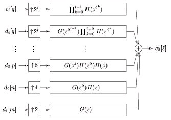


Recall the iterated synthesis filterbank. Applying the Noble identities, we can move the up-
samplers before the filters, as illustrated in Figure 4.30.
Figure 4.30.
The properties of the i-stage cascaded lowpass filter
()
in the limit i→∞ give an important characterization of the wavelet system. But how do we know
that
converges to a response in ℒ 2 ? In fact, there are some rather strict conditions on
H( ⅇⅈω) that must be satisfied for this convergence to occur. Without such convergence, we might
have a finite-stage perfect reconstruction filterbank, but we will not have a countable wavelet
basis for ℒ 2 . Below we present some "regularity conditions" on H( ⅇⅈω) that ensure convergence of the iterated synthesis lowpass filter.
The convergence of the lowpass filter implies convergence of all other filters in the bank.
Let us denote the impulse response of H ( i ) ( z) by h ( i ) [ n] . Writing
H ( i ) ( z)= H( z 2 i−1) H ( i − 1 ) ( z) in the time domain, we have Now define
the function
where ℐ [ a , b ) ( t) denotes the indicator function over
the interval [ a, b) :
The definition of φ ( i ) ( t) implies
()
()


and plugging the two previous expressions into the equation for h ( i ) [ n] yields
()
Thus, if φ ( i ) ( t) converges pointwise to a continuous function, then it must satisfy the scaling
equation, so that
. Daubechies [link] showed that, for pointwise convergence of
φ ( i ) ( t) to a continuous function in ℒ 2 , it is sufficient that H( ⅇⅈω) can be factored as ()
for R( ⅇⅈω) such that
()
Here P denotes the number of zeros that H( ⅇⅈω) has at ω= π . Such conditions are called regularity conditions because they ensure the regularity, or smoothness of φ( t) . In fact, if we make the
previous condition stronger:
()
then
for φ( t) that is ℓ-times continuously differentiable.
There is an interesting and important by-product of the preceding analysis. If h[ n] is a causal
length- N filter, it can be shown that h ( i ) [ n] is causal with length Ni=(2 i−1)( N−1)+1 . By construction, then, φ ( i ) [ t] will be zero outside the interval
. Assuming that the
regularity conditions are satisfied so that
, it follows that φ( t) must be zero outside
the interval [0, N−1] . In this case we say that φ( t) has compact support. Finally, the wavelet
scaling equation implies that, when φ( t) is compactly supported on [0, N−1] and g[ n] is length N, ψ( t) will also be compactly supported on the interval [0, N−1] .
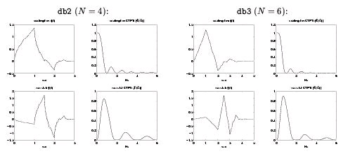
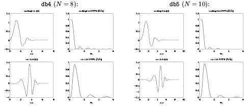
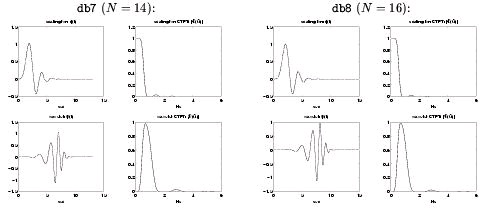
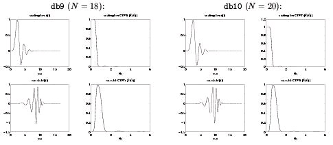
Daubechies constructed a family of H( z) with impulse response lengths N∈{4, 6, 8, 10, …} which
satisfy the regularity conditions. Moreover, her filters have the maximum possible number of
zeros at ω= π , and thus are maximally regular (i.e., they yield the smoothest possible φ( t) for a given support interval). It turns out that these filters are the maximally flat filters derived by
Herrmann [link] long before filterbanks and wavelets were in vogue. In Figure 4.31 and
Figure 4.32 we show φ( t) , Φ( Ω) , ψ( t) , and Ψ( Ω) for various members of the Daubechies' wavelet system.
See Vetterli and Kovacivić [link] for a more complete discussion of these matters.
(a)
(b)
Figure 4.31.
(a)
(b)


Figure 4.32.
References
1. I. Daubechies. (1988, Nov). Orthonormal bases of compactly supported wavelets. Commun. on
Pure and Applied Math, 41, 909-996.
2. O. Herrmann. (1971). On the approximation problem in nonrecursive digital filter design.
IEEE Trans. on Circuit Theory, 18, 411-413.
3. M. Vetterli and J. Kovacivić. (1995). Wavelets and Subband Coding. Englewood Cliffs, NJ:
Prentice Hall.
Computing the Scaling Function: The Cascade Algorithm*
Given coefficients { h[ n]} that satisfy the regularity conditions, we can iteratively calculate
samples of φ( t) on a fine grid of points { t} using the cascade algorithm. Once we have obtained
φ( t) , the wavelet scaling equation can be used to construct ψ( t) .
In this discussion we assume that H( z) is causal with impulse response length N. Recall, from our
discussion of the regularity conditions, that this implies φ( t) will have compact support on the interval [0, N−1] . The cascade algorithm is described below.
1. Consider the scaling function at integer times t= m∈{0, …, N−1} :
Knowing that φ( t)=0 for t∉[0, N−1] , the previous equation can be written using an N x N
matrix. In the case where N=4 , we have
()
The matrix H is structured as a row-decimated convolution matrix.
From the matrix equation above (Equation), we see that ( φ(0), φ(1), φ(2), φ(3)) T must be (some scaled version of) the eigenvector of H corresponding to eigenvalue
. In general,
the nonzero values of { φ( n)| n∈ℤ} , i.e. , ( φ(0), φ(1), …, φ( N−1)) T , can be calculated by appropriately scaling the eigenvector of the N x N row-decimated convolution matrix H
corresponding to the eigenvalue
. It can be shown that this eigenvector must be scaled so
that
.
2. Given { φ( n)| n∈ℤ} , we can use the scaling equation to determine
:


2. Given { φ( n)| n∈ℤ} , we can use the scaling equation to determine
:
()
This produces the 2 N−1 non-zero samples { φ(0), φ(1/2), φ(1), φ(3/2), …, φ( N−1)} .
3. Given
, the scaling equation can be used to find
:
()
where h ↑ 2 [ p] denotes the impulse response of H( z 2) , i.e. , a 2-upsampled version of h[ n] , and where
. Note that
is the result of convolving h ↑ 2 [ n] with
.
4. Given
, another convolution yields
:
()
where h ↑ 4 [ n] is a 4-upsampled version of h[ n] and where
.
5. At the ℓ th stage,
is calculated by convolving the result of the ℓ − 1 th stage with a 2 ℓ−1 -
upsampled version of h[ n] :
()
For ℓ≈10 , this gives a very good approximation of φ( t) . At this point, you could verify the key
properties of φ( t) , such as orthonormality and the satisfaction of the scaling equation.
In Figure 4.33 we show steps 1 through 5 of the cascade algorithm, as well as step 10, using
Daubechies' db2 coefficients (for which N=4 ).
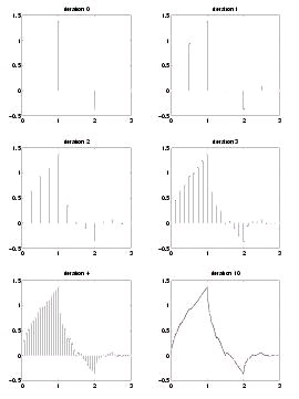
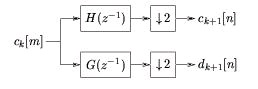


Figure 4.33.
Finite-Length Sequences and the DWT Matrix*
The wavelet transform, viewed from a filterbank perspective, consists of iterated 2-channel
analysis stages like the one in Figure 4.34.
Figure 4.34.
First consider a very long (i.e., practically infinite-length) sequence