The classical theory behind the encoding analog signals into bit streams and decoding bit streams back into signals, rests on a famous sampling theorem which is typically refereed to as the Shannon-Whitaker Sampling Theorem. In this course, this sampling theory will serve as a benchmark to which we shall compare the new theory of compressed sensing.
To introduce the Shannon-Whitaker theory, we first define the class of bandlimited signals. A bandlimited signal is a signal whose Fourier transform only has finite support. We shall denote this class as BA and define it in the following way:

Here, the Fourier transform of f is defined by

This formula holds for any f∈L1 and extends easily to f∈L2 via limits. The inversion of the Fourier transform is given by

<ext:rule>
If f∈BA, then f can be uniquely determined by the
uniformly spaced samples  and in fact,
is given by
and in fact,
is given by

where  .
.
It is enough to consider A=1, since all other cases can be reduced to this through a simple change of variables. Because f∈BA=1, the Fourier inversion formula takes the form

Define F(ω) as the 2π periodization of  ,
,

Because F(ω) is periodic, it admits a Fourier series representation

where the Fourier coefficients cn given by

By comparing (Equation) with (Equation), we conclude that

Therefore by plugging (Equation) back into (Equation), we have that

Now, because

and because of the facts that

we conclude

Comments:
(Good news) The set  is an orthogonal system and therefore, has the property that the L2 norm of the function and its Fourier coefficients are related by,

(Bad news) The representation of f in terms of sinc functions is not a stable representation, i.e.

To fix the instability of the Shannon representation, we assume that the signal is slightly more bandlimited than before

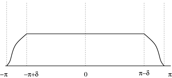
and instead of using χ[–π,π], we multiply by another
function  which is very similar in form to the
characteristic function, but decays at its boundaries in a smoother
fashion (i.e. it has more derivatives). A candidate function
is sketched in Figure 1.1.
which is very similar in form to the
characteristic function, but decays at its boundaries in a smoother
fashion (i.e. it has more derivatives). A candidate function
is sketched in Figure 1.1.
 .
.
Now, it is a property of the Fourier transform that an increased
smoothness in one domain translates into a faster decay in the
other. Thus, we can fix our instability problem, by choosing
 so that is smooth and
  , |ω|≤π–δ
and , |ω|>π. By choosing the smoothness of g suitably large, we can, for any given m≥1, choose g to satisfy
, |ω|≤π–δ
and , |ω|>π. By choosing the smoothness of g suitably large, we can, for any given m≥1, choose g to satisfy
for some constant C>0.
Using such a  , we can rewrite (???)
as
, we can rewrite (???)
as
Thus, we have the new representation
where we gain stability from our additional assumption that the signal is bandlimited on [–π–δ,π–δ].
Does this assumption really hurt? No, not really because if our signal is really bandlimited to [–π,π] and not [–π–δ,π–δ], we can always take a slightly larger bandwidth, say [–λπ,λπ] where λ is a little larger than one, and carry out the same analysis as above. Doing so, would only mean slightly oversampling the signal (small cost).
Recall that in the end we want to convert analog signals into bit streams. Thus far, we have the two representations
Shannon's Theorem tells us that if f∈BA, we should
sample f at the Nyquist rate A (which is twice the support of ) and then take the binary
representation of the samples. Our more stable representation says
to slightly oversample f and then convert to a binary
representation. Both representations offer perfect reconstruction,
although in the more stable representation, one is straddled with
the additional task of choosing an appropriate λ.
In practical situations, we shall be interested in approximating f on an interval [–T,T] for some T>0 and not for all time. Questions we still want to answer include
How many bits do we need to represent f in BA=1 on some interval [–T,T] in the norm L∞[–T,T]?
Using this methodology, what is the optimal way of encoding?
How is the optimal encoding implemented?
Towards this end, we define

Then for any f∈BA, we can write

In other words, samples at 0,  ,
,  are sufficient to reconstruct f. Recall also
that
are sufficient to reconstruct f. Recall also
that  decays poorly
(leading to numerical instability). We can overcome this problem by
slight over-sampling. Say we over-sample by a factor λ>1.
Then, we can write
decays poorly
(leading to numerical instability). We can overcome this problem by
slight over-sampling. Say we over-sample by a factor λ>1.
Then, we can write

Hence we need samples at 0,  ,
,  , etc.
What is the advantage? Sampling more often than necessary buys us stability because we now have a choice
for gλ(·).
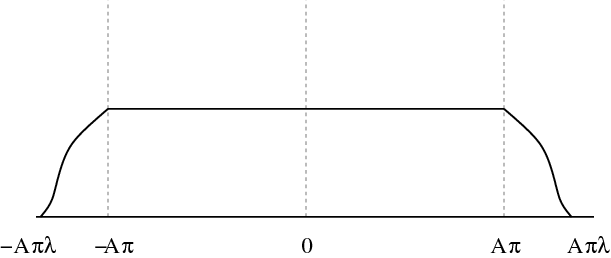
If we choose gλ(·) infinitely differentiable whose Fourier transform looks
as shown in Figure 1.2 we can obtain
, etc.
What is the advantage? Sampling more often than necessary buys us stability because we now have a choice
for gλ(·).
If we choose gλ(·) infinitely differentiable whose Fourier transform looks
as shown in Figure 1.2 we can obtain

and therefore gλ(·) decays very fast. In other words, a sample's influence is felt only locally. Note however, that over-sampling generates basis functions that are redundant (linearly dependent), unlike the integer translates of the sinc(·) function.

If we restrict our reconstruction to t in the interval [–T,T], we will only need samples only from [–cT,cT], for c>1 (see Figure 1.3), because the distant samples will have little effect on the reconstruction in [–T,T].
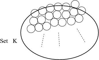
We shall consider now the encoding of signals on [–T,T] where T>0 is fixed. Ultimately we shall be interested in encoding classes of bandlimited signals like the class BA However, we begin the story by considering the more general setting of encoding the elements of any given compact subset K of a normed linear space X. One can determine the best encoding of K by what is known as the Kolmogorov entropy of K in X.
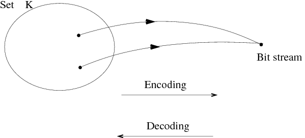
To begin, let us consider an encoder-decoder pair (E,D) E maps K to a finite stream of bits. D maps a stream of bits to a signal in X. This is illustrated in Figure 1.4. Note that many functions can be mapped onto the same bitstream.
Define the distortion d for this encoder-decoder by
Let  where
#Ef is the number of bits
in the bitstream Ef.
Thus n is the maximum
length of the bitstreams for the various f∈K. There are two ways we can
define optimal encoding:
where
#Ef is the number of bits
in the bitstream Ef.
Thus n is the maximum
length of the bitstreams for the various f∈K. There are two ways we can
define optimal encoding:
Prescribe ϵ, the maximum distortion that
we are willing to tolerate. For this ϵ, find the smallest
. This is the smallest bit budget under which we could encode all elements of K to distortion ϵ.
Prescribe N : find the smallest distortion d(K,E,D,X) over all E,D with n(K,E)≤N. This is the best encoding performance possible with a prescribed bit budget.
There is a simple mathematical solution to these two encoding problems based on the notion of Kolmogorov Entropy.