For much of its history, signal processing has focused on signals produced by physical systems. Many natural and man-made systems can be modeled as linear. Thus, it is natural to consider signal models that complement this kind of linear structure. This notion has been incorporated into modern signal processing by modeling signals as vectors living in an appropriate vector space. This captures the linear structure that we often desire, namely that if we add two signals together then we obtain a new, physically meaningful signal. Moreover, vector spaces allow us to apply intuitions and tools from geometry in R³, such as lengths, distances, and angles, to describe and compare signals of interest. This is useful even when our signals live in high-dimensional or infinite-dimensional spaces.

Throughout this course, we will treat signals as real-valued functions having domains that are either continuous or discrete, and either infinite or finite. These assumptions will be made clear as necessary in each chapter. In this course, we will assume that the reader is relatively comfortable with the key concepts in vector spaces. We now provide only a brief review of some of the key concepts in vector spaces that will be required in developing the theory of compressive sensing (CS). For a more thorough review of vector spaces see this introductory course in Digital Signal Processing.

We will typically be concerned with normed vector spaces, i.e., vector spaces endowed with a norm. In the case of a discrete, finite domain, we can view our signals as vectors in an N-dimensional Euclidean space, denoted by R^N. When dealing with vectors in R^N, we will make frequent use of the ℓ_p norms, which are defined for p∈[1,∞] as

(2.1)

In Euclidean space we can also consider the standard inner product in R^N, which we denote

(2.2)

This inner product leads to the ℓ₂ norm: .

In some contexts it is useful to extend the notion of ℓ_p norms to the case where p<1. In this case, the “norm” defined in Equation 2.1 fails to satisfy the triangle inequality, so it is actually a quasinorm. We will also make frequent use of the notation ∥x∥₀:=| supp (x)|, where denotes the support of x and | supp (x)| denotes the cardinality of supp (x). Note that ∥·∥₀ is not even a quasinorm, but one can easily show that

(2.3)

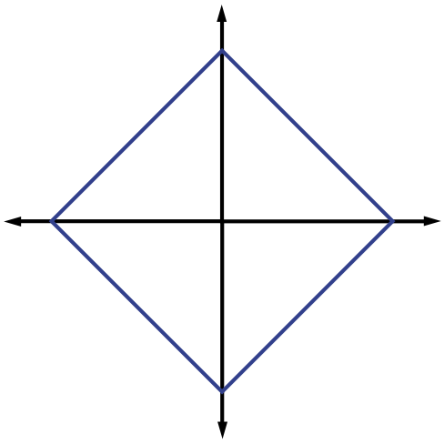
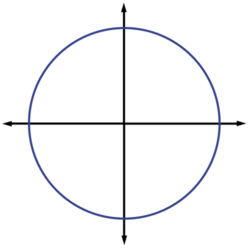
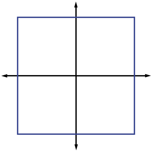
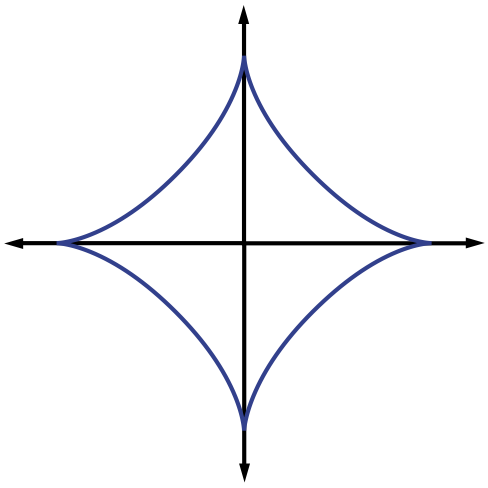
justifying this choice of notation. The ℓ_p (quasi-)norms have notably different properties for different values of p. To illustrate this, in Figure 2.1 we show the unit sphere, i.e., induced by each of these norms in R². Note that for p<1 the corresponding unit sphere is nonconvex (reflecting the quasinorm's violation of the triangle inequality).

(a) Unit sphere for ℓ1 norm

(b) Unit sphere for ℓ2 norm

(c) Unit sphere for ℓ∞ norm

(d) Unit sphere for ℓp quasinorm

Figure 2.1. 

Unit spheres in R² for the ℓ_p norms with p=1,2,∞, and for the ℓ_p quasinorm with .

We typically use norms as a measure of the strength of a signal, or the size of an error. For example, suppose we are given a signal x∈R² and wish to approximate it using a point in a one-dimensional affine space A. If we measure the approximation error using an ℓ_p norm, then our task is to find the that minimizes . The choice of p will have a significant effect on the properties of the resulting approximation error. An example is illustrated in Figure 2.2. To compute the closest point in A to x using each ℓ_p norm, we can imagine growing an ℓ_p sphere centered on x until it intersects with A. This will be the point that is closest to x in the corresponding ℓ_p norm. We observe that larger p tends to spread out the error more evenly among the two coefficients, while smaller p leads to an error that is more unevenly distributed and tends to be sparse. This intuition generalizes to higher dimensions, and plays an important role in the development of CS theory.

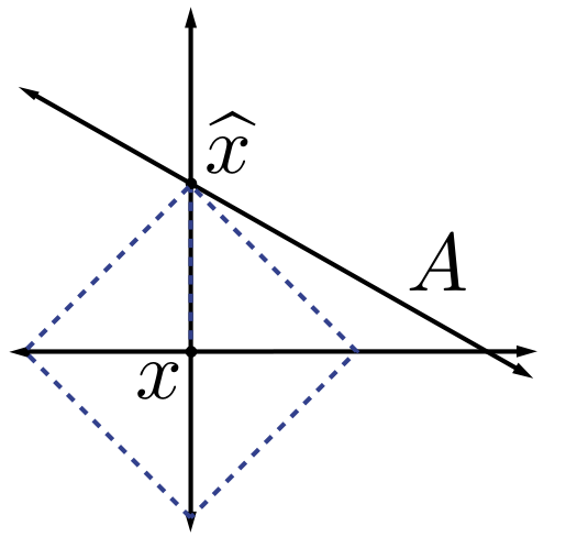(a) Approximation in ℓ1 norm

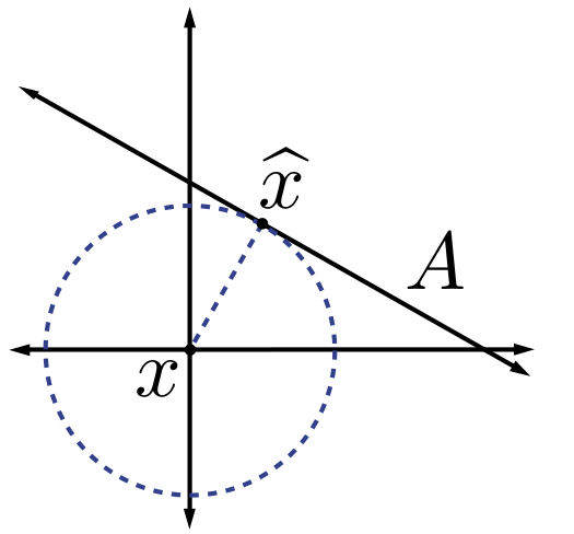(b) Approximation in ℓ2 norm

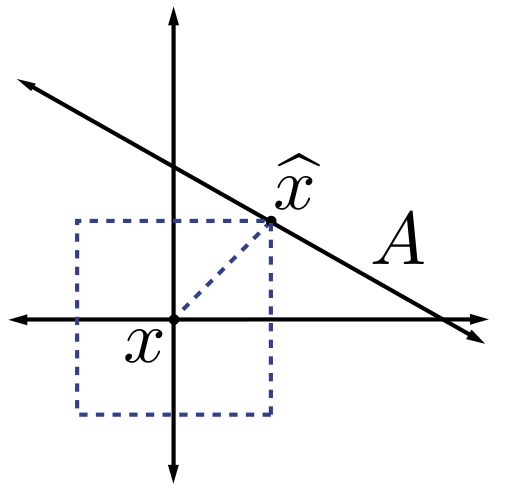(c) Approximation in ℓ∞ norm

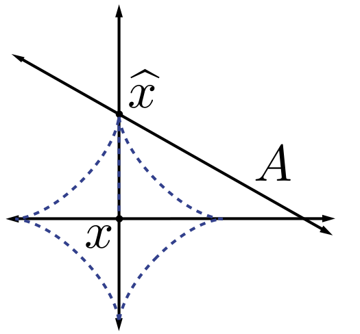(d) Approximation in ℓp quasinorm

Figure 2.2. 

Best approximation of a point in R² by a a one-dimensional subspace using the ℓ_p norms for p=1,2,∞, and the ℓ_p quasinorm with .

A set is called a basis for a finite-dimensional vector space V if the vectors in the set span V and are linearly independent. This implies that each vector in the space can be represented as a linear combination of this (smaller, except in the trivial case) set of basis vectors in a unique fashion. Furthermore, the coefficients of this linear combination can be found by the inner product of the signal and a dual set of vectors. In discrete settings, we will only consider real finite-dimensional Hilbert spaces where V=R^N and I={1,...,N}.

Mathematically, any signal x∈R^N may be expressed as,

(2.4)

where our coefficients are computed as a_i=〈x,ψ_i〉 and are the vectors that constitute our dual basis. Another way to denote our basis and its dual is by how they operate on x. Here, we call our dual basis our synthesis basis (used to reconstruct our signal by Equation 2.4) and Ψ is our analysis basis.

An orthonormal basis (ONB) is defined as a set of vectors that form a basis and whose elements are orthogonal and unit norm. In other words, 〈ψ_i,ψ_j〉=0 if i≠j and one otherwise. In the case of an ONB, the synthesis basis is simply the Hermitian adjoint of analysis basis ().

It is often useful to generalize the concept of a basis to allow for sets of possibly linearly dependent vectors, resulting in what is known as a frame. More formally, a frame is a set of vectors in R^d, d<n corresponding to a matrix Ψ∈R^d×n, such that for all vectors x∈R^d,

with 0<A≤B<∞. Note that the condition A>0 implies that the rows of Ψ must be linearly independent. When A is chosen as the largest possible value and B as the smallest for these inequalities to hold, then we call them the (optimal) frame bounds. If A and B can be chosen as A=B, then the frame is called A-tight, and if A=B=1, then Ψ is a Parseval frame. A frame is called equal-norm, if there exists some λ>0 such that ∥Ψ_i∥₂=λ for all i=1,...,N, and it is unit-norm if λ=1. Note also that while the concept of a frame is very general and can be defined in infinite-dimensional spaces, in the case where Ψ is a d×N matrix A and B simply correspond to the smallest and largest eigenvalues of ΨΨ^T, respectively.

Frames can provide richer representations of data due to their redundancy: for a given signal x, there exist infinitely many coefficient vectors α such that x=Ψα. In particular, each choice of a dual frame provides a different choice of a coefficient vector α. More formally, any frame satisfying

(2.6)

is called an (alternate) dual frame. The particular choice is referred to as the canonical dual frame. It is also known as the Moore-Penrose pseudoinverse. Note that since A>0 requires Ψ to have linearly independent rows, we ensure that ΨΨ^T is invertible, so that is well-defined. Thus, one way to obtain a set of feasible coefficients is via

(2.7)

One can show that this sequence is the smallest coefficient sequence in ℓ₂ norm, i.e., ∥α_d∥₂≤∥α∥₂ for all α such that x=Ψα.

Finally, note that in the sparse approximation literature, it is also common for a basis or frame to be referred to as a dictionary or overcomplete dictionary respectively, with the dictionary elements being called atoms.

Transforming a signal to a new basis or frame may allow us to represent a signal more concisely. The resulting compression is useful for reducing data storage and data transmission, which can be quite expensive in some applications. Hence, one might wish to simply transmit the analysis coefficients obtained in our basis or frame expansion instead of its high-dimensional correlate. In cases where the number of non-zero coefficients is small, we say that we have a sparse representation. Sparse signal models allow us to achieve high rates of compression and in the case of compressive sensing, we may use the knowledge that our signal is sparse in a known basis or frame to recover our original signal from a small number of measurements. For sparse data, only the non-zero coefficients need to be stored or transmitted in many cases; the rest can be assumed to be zero).

Mathematically, we say that a signal x is K-sparse when it has at most K nonzeros, i.e., ∥x∥₀≤K. We let

denote the set of all K-sparse signals. Typically, we will be dealing with signals that are not themselves sparse, but which admit a sparse representation in some basis Ψ. In this case we will still refer to x as being K