Random variables whose spaces are not composed of a countable number of points but are intervals or a union of intervals are said to be of the continuous type. Recall that the relative frequency histogram h( x ) associated with n observations of a random variable of that type is a nonnegative function defined so that the total area between its graph and the x axis equals one. In addition, h( x ) is constructed so that the integral

is an estimate of the probability P( a<X<b ) , where the interval ( a,b ) is a subset of the space R of the random variable X.
Let now consider what happens to the function h( x ) in the limit, as n increases without bound and as the lengths of the class intervals decrease to zero. It is to be hoped that h( x ) will become closer and closer to some function, say f( x ) , that gives the true probabilities , such as P( a<X<b ) , through the integral

1. Function f(x) is a nonnegative function such that the total area between its graph and the x axis equals one.
2. The probability P( a<X<b ) is the area bounded by the graph of f( x ) , the x axis, and the lines x=a and x=b .
3. We say that the probability density function (p.d.f.) of the random variable X of the continuous type, with space R that is an interval or union of intervals, is an integrable function f( x ) satisfying the following conditions:
f( x )>0 , x belongs to R,

The probability of the event A belongs to R is 
Let the random variable X be the distance in feet between bad records on a used computer tape. Suppose that a reasonable probability model for X is given by the p.d.f.


The probability that the distance between bad records is greater than 40 feet is

The p.d.f. and the probability of interest are depicted in FIG.1.

We can avoid repeated references to the space R of the random variable X, one shall adopt the same convention when describing probability density function of the continuous type as was in the discrete case.
Let extend the definition of the p.d.f. f( x ) to the entire set of real numbers by letting it equal zero when, x belongs to R. For example,

has the properties of a p.d.f. of a continuous-type random variable x having support ( x:0≤x<∞ ) . It will always be understood that f(x)=0 , when x belongs to R, even when this is not explicitly written out.
1.
The distribution function of a random variable X of the continuous type, is defined in terms of the p.d.f. of X, and is given by 
2. For the fundamental theorem of calculus we have, for x values for which the derivative F'( x ) exists, that F’(x)=f(x).
continuing with Example 1
If the p.d.f. of X is

The distribution function of X is F( x )=0 for x≤0


Also F'( 0 ) does not exist. Since there are no steps or jumps in a distribution function F( x ) , of the continuous type, it must be true that P( X=b )=0 for all real values of b. This agrees with the fact that the integral
 is taken to be zero in calculus. Thus we see that
P(
a≤X≤b
)=P(
a<X<b
)=P(
a≤X<b
)=P(
a<X≤b
)=F(
b
)−F(
a
),
provided that X is a random variable of the continuous type. Moreover, we can change the definition of a p.d.f. of a random variable of the continuous type at a finite (actually countable) number of points without alerting the distribution of probability.
is taken to be zero in calculus. Thus we see that
P(
a≤X≤b
)=P(
a<X<b
)=P(
a≤X<b
)=P(
a<X≤b
)=F(
b
)−F(
a
),
provided that X is a random variable of the continuous type. Moreover, we can change the definition of a p.d.f. of a random variable of the continuous type at a finite (actually countable) number of points without alerting the distribution of probability.
For illustration,  and
and 
are equivalent in the computation of probabilities involving this random variable.
Let Y be a continuous random variable with the p.d.f. g( y )=2y , 0<y<1 . The distribution function of Y is defined by

Figure 2 gives the graph of the p.d.f. g( y ) and the graph of the distribution function G( y ) .

For illustration of computations of probabilities, consider

and 
The p.d.f. f( x ) of a random variable of the discrete type is bounded by one because f( x ) gives a probability, namely f( x )=P( X=x ) .
For random variables of the continuous type, the p.d.f. does not have to be bounded. The restriction is that the area between the p.d.f. and the x axis must equal one. Furthermore, it should be noted that the p.d.f. of a random variable X of the continuous type does not need to be a continuous function.

enjoys the properties of a p.d.f. of a distribution of the continuous type, and yet f( x ) had discontinuities at x=0,1,2, and 3. However, the distribution function associates with a distribution of the continuous type is always a continuous function. For continuous type random variables, the definitions associated with mathematical expectation are the same as those in the discrete case except that integrals replace summations.
Let the random variable X denote the outcome when a point is selected at random from the interval [ a,b ] , −∞<a<b<∞ . If the experiment is performed in a fair manner, it is reasonable to assume that the probability that the point is selected from the interval [ a,x ] , a≤x<b is ( x−a )( b−a ) . That is, the probability is proportional to the length of the interval so that the distribution function of X is

Because X is a continuous-type random variable, F'( x ) is equal to the p.d.f. of X whenever F'( x ) exists; thus when a<x<b , we have f( x )=F'( x )=1/( b−a ).
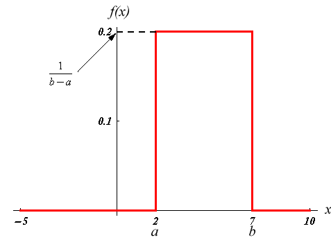
The random variable X has a uniform distribution if its p.d.f. is equal to a constant on its support. In particular, if the support is the interval [ a,b ] , then

Moreover, one shall say that X is U( a,b ) . This distribution is referred to as rectangular because the graph of f( x ) suggest that name. See Figure1. for the graph of f( x ) and the distribution function F(x).
We could have taken f( a )=0 or f( b )=0 without alerting the probabilities, since this is a continuous type distribution, and it can be done in some cases.
The mean and variance of X are as follows:
and
An important uniform distribution is that for which a=0 and b =1, namely U( 0,1 ) . If X is U( 0,1 ) , approximate values of X can be simulated on most computers using a random number generator. In fact, it should be called a pseudo-random number generator (see the pseudo-numbers generation) because the programs that produce the random numbers are usually such that if the starting number is known, all subsequent numbers in the sequence may be determined by simple arithmetical op