Bank A:
012
.
0
APY = 1
+
−1 = 01205
.
0
4 = 1.2054%
4
12
Bank B:
0 011
.
APY = 1
+
−1 = 01105
.
0
6 = 1.1056%
12
Bank B’s monthly compounding is not enough to catch up with Bank A’s better APR.
Bank A offers a better rate.
A Limit to Compounding
As we saw earlier, the amount we earn increases as we increase the compounding
frequency. The table, though, shows that the increase from annual to semi-annual
compounding is larger than the increase from monthly to daily compounding. This might
lead us to believe that although increasing the frequency of compounding will increase
our result, there is an upper limit to this process.
Section 4.1 Exponential Functions 225
To see this, let us examine the value of $1 invested at 100% interest for 1 year.
Frequency
Value
Annual
$2
Semiannually
$2.25
Quarterly
$2.441406
Monthly
$2.613035
Daily
$2.714567
Hourly
$2.718127
Once per minute
$2.718279
Once per second
$2.718282
These values do indeed appear to be approaching an upper limit. This value ends up
being so important that it gets represented by its own letter, much like how π represents a
number.
Euler’s Number: e
k
e is the letter used to represent the value that
+ 1
1
approaches as k gets big.
k
e ≈ 718282
.
2
Because e is often used as the base of an exponential, most scientific and graphing
calculators have a button that can calculate powers of e, usually labeled ex. Some
computer software instead defines a function exp(x), where exp(x) = ex.
Because e arises when the time between compounds becomes very small, e allows us to
define continuous growth and allows us to define a new toolkit function, ( )
x
f x = e .
Continuous Growth Formula
Continuous Growth can be calculated using the formula
rx
f ( x) = ae
where
a is the starting amount
r is the continuous growth rate
This type of equation is commonly used when describing quantities that change more or
less continuously, like chemical reactions, growth of large populations, and radioactive
decay.
226 Chapter 4
Example 11
Radon-222 decays at a continuous rate of 17.3% per day. How much will 100mg of
Radon-222 decay to in 3 days?
Since we are given a continuous decay rate, we use the continuous growth formula.
Since the substance is decaying, we know the growth rate will be negative: r = -0.173
f )
3
( = 100 − 173
.
0
(3)
e
≈
512
.
59
mg of Radon-222 will remain.
Try it Now
6. Interpret the following:
0.12
( ) = 20
t
S t
e
if S(t) represents the growth of a substance in
grams, and time is measured in days.
Continuous growth is also often applied to compound interest, allowing us to talk about
continuous compounding.
Example 12
If $1000 is invested in an account earning 10% compounded continuously, find the
value after 1 year.
Here, the continuous growth rate is 10%, so r = 0.10. We start with $1000, so a = 1000.
To find the value after 1 year,
f )
1
( = 1000 10
.
0
)
1
(
e
≈
17
.
1105
$
Notice this is a $105.17 increase for the year. As a percent increase, this is
105 17
.
= 1051
.
0
7 =
%
517
.
10
increase over the original $1000.
1000
Notice that this value is slightly larger than the amount generated by daily compounding
in the table computed earlier.
The continuous growth rate is like the nominal growth rate (or APR) – it reflects the
growth rate before compounding takes effect. This is different than the annual growth
rate used in the formula
x
f ( x) = a 1
( + r) , which is like the annual percentage yield – it
reflects the actual amount the output grows in a year.
While the continuous growth rate in the example above was 10%, the actual annual yield
was 10.517%. This means we could write two different looking but equivalent formulas
for this account’s growth:
0.10
( ) =1000
t
f t
e
using the 10% continuous growth rate
( ) 1000(1.10517) t
f t =
using the 10.517% actual annual yield rate.
Section 4.1 Exponential Functions 227
Important Topics of this Section
Percent growth
Exponential functions
Finding formulas
Interpreting equations
Graphs
Exponential Growth & Decay
Compound interest
Annual Percent Yield
Continuous Growth
Try it Now Answers
1. A & C are exponential functions, they grow by a % not a constant number.
2. B(t) is growing faster, but after 3 years A(t) still has a higher account balance
3.
(
1000 0 97
. )30 =
0071
.
401
4. f ( ) = (
2 1 5
. ) x
x
5. $1024.25
6. An initial substance weighing 20g is growing at a continuous rate of 12% per day.
228 Chapter 4
Section 4.1 Exercises
For each table below, could the table represent a function that is linear, exponential, or
neither?
1.
x 1 2 3 4
2.
x 1 2 3 4
g(x) 40 32 26 22
f(x) 70 40 10 -20
3.
x 1 2 3
4
4.
x 1 2 3 4
k(x) 90 80 70 60
h(x) 70 49 34.3 24.01
5.
x
1 2 3
4
6.
x 1 2 3
4
m(x) 80 61
n(x) 90 81 72.9 65.61
42.9 25.61
7. A population numbers 11,000 organisms initially and grows by 8.5% each year.
Write an exponential model for the population.
8. A population is currently 6,000 and has been increasing by 1.2% each day. Write an
exponential model for the population.
9. The fox population in a certain region has an annual growth rate of 9 percent per year.
It is estimated that the population in the year 2010 was 23,900. Estimate the fox
population in the year 2018.
10. The amount of area covered by blackberry bushes in a park has been growing by 12%
each year. It is estimated that the area covered in 2009 was 4,500 square feet.
Estimate the area that will be covered in 2020.
11. A vehicle purchased for $32,500 depreciates at a constant rate of 5% each year.
Determine the approximate value of the vehicle 12 years after purchase.
12. A business purchases $125,000 of office furniture which depreciates at a constant rate
of 12% each year. Find the residual value of the furniture 6 years after purchase.
Section 4.1 Exponential Functions 229
Find a formula for an exponential function passing through the two points.
13. (0, 6), (3, 750)
14. (0, 3), (2, 75)
15. (0, 2000), (2, 20)
16. (0, 9000), (3, 72)
17.
3
1,
−
2
,( 3, 24)
18. 1,
−
,( 1,10)
2
5
19. ( 2
− ,6),( 3, )
1
20. ( 3
− ,4), (3, 2)
21. (3, )
1 , (5, 4)
22. (2,5), (6, 9)
23. A radioactive substance decays exponentially. A scientist begins with 100 milligrams
of a radioactive substance. After 35 hours, 50 mg of the substance remains. How
many milligrams will remain after 54 hours?
24. A radioactive substance decays exponentially. A scientist begins with 110 milligrams
of a radioactive substance. After 31 hours, 55 mg of the substance remains. How
many milligrams will remain after 42 hours?
25. A house was valued at $110,000 in the year 1985. The value appreciated to $145,000
by the year 2005. What was the annual growth rate between 1985 and 2005?
Assume that the house value continues to grow by the same percentage. What did the
value equal in the year 2010?
26. An investment was valued at $11,000 in the year 1995. The value appreciated to
$14,000 by the year 2008. What was the annual growth rate between 1995 and 2008?
Assume that the value continues to grow by the same percentage. What did the value
equal in the year 2012?
27. A car was valued at $38,000 in the year 2003. The value depreciated to $11,000 by
the year 2009. Assume that the car value continues to drop by the same percentage.
What will the value be in the year 2013?
28. A car was valued at $24,000 in the year 2006. The value depreciated to $20,000 by
the year 2009. Assume that the car value continues to drop by the same percentage.
What will the value be in the year 2014?
29. If $4,000 is invested in a bank account at an interest rate of 7 per cent per year, find
the amount in the bank after 9 years if interest is compounded annually, quarterly,
monthly, and continuously.
230 Chapter 4
30. If $6,000 is invested in a bank account at an interest rate of 9 per cent per year, find
the amount in the bank after 5 years if interest is compounded annually, quarterly,
monthly, and continuously.
31. Find the annual percentage yield (APY) for a savings account with annual percentage
rate of 3% compounded quarterly.
32. Find the annual percentage yield (APY) for a savings account with annual percentage
rate of 5% compounded monthly.
33. A population of bacteria is growing according to the equation
0.21
( ) =1 600
t
P t
e
, with t
measured in years. Estimate when the population will exceed 7569.
34. A population of bacteria is growing according to the equation
0.17
( ) =1 200
t
P t
e
, with t
measured in years. Estimate when the population will exceed 3443.
35. In 1968, the U.S. minimum wage was $1.60 per hour. In 1976, the minimum wage
was $2.30 per hour. Assume the minimum wage grows according to an exponential
model (
w t) , where t represents the time in years after 1960. [UW]
a. Find a formula for (
w t) .
b. What does the model predict for the minimum wage in 1960?
c. If the minimum wage was $5.15 in 1996, is this above, below or equal to what
the model predicts?
36. In 1989, research scientists published a model for predicting the cumulative number
3
−
of AIDS cases (in thousands) reported in the United States: a( t)
t 1980
155
=
,
10
where t is the year. This paper was considered a “relief”, since there was a fear the
correct model would be of exponential type. Pick two data points predicted by the
research model a( t) to construct a new exponential model b( t) for the number of cumulative AIDS cases. Discuss how the two models differ and explain the use of the
word “relief.” [UW]

Section 4.1 Exponential Functions 231
37. You have a chess board as pictured, with
squares numbered 1 through 64. You also have
a huge change jar with an unlimited number of
dimes. On the first square you place one dime.
On the second square you stack 2 dimes. Then
you continue, always doubling the number
from the previous square. [UW]
a. How many dimes will you have
stacked on the 10th square?
b. How many dimes will you have
stacked on the nth square?
c. How many dimes will you have
stacked on the 64th square?
d. Assuming a dime is 1 mm thick, how
high will this last pile be?
e. The distance from the earth to the sun is approximately 150 million km.
Relate the height of the last pile of dimes to this distance.
232 Chapter 4
Section 4.2 Graphs of Exponential Functions
Like with linear functions, the graph of an exponential function is determined by the
values for the parameters in the function’s formula.
To get a sense for the behavior of exponentials, let us begin by looking more closely at
the function
x
f ( x) = 2 . Listing a table of values for this function:
x
-3
-2
-1
0
1
2
3
f(x)
1
1
1
1
2
4
8
8
4
2
Notice that:
1) This function is positive for all values of x.
2) As x increases, the function grows faster and faster (the rate of change
increases).
3) As x decreases, the function values grow smaller, approaching zero.
4) This is an example of exponential growth.
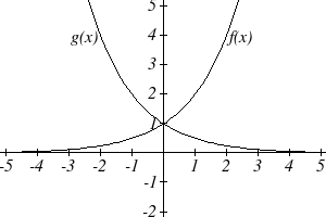
x
Looking at the function g( x
1
) =
2
x
-3
-2
-1
0
1
2
3
g(x)
8
4
2
1
1
1
1
2
4
8
Note this function is also positive for all values of x, but in this case grows as x decreases, and decreases towards zero as x increases. This is an example of exponential decay. You
may notice from the table that this function appears to be the horizontal reflection of the
x
f ( x) = 2 table. This is in fact the case:
x
− x
1
−
x
1
f (− x) = 2 = (2 )
= = g( x)
2
Looking at the graphs also confirms this relationship:
Section 4.2 Graphs of Exponential Functions 233
Consider a function for the form
x
f ( x) = ab . Since a, which we called the initial value
in the last section, is the function value at an input of zero, a will give us the vertical
intercept of the graph. From the graphs above, we can see that an exponential graph will
have a horizontal asymptote on one side of the graph, and can either increase or decrease,
depending upon the growth factor. This horizontal asymptote will also help us determine
the long run behavior and is easy to determine from the graph.
The graph will grow when the growth rate is positive, which will make the growth factor
b larger than one. When it’s negative, the growth factor will be less than one.
Graphical Features of Exponential Functions
Graphically, in the function
x
f ( x) = ab
a is the vertical intercept of the graph
b determines the rate at which the graph grows
the function will increase if b > 1
the function will decrease if 0 < b < 1
The graph will have a horizontal asymptote at y = 0
The graph will be concave up if a > 0; concave down if a < 0.
The domain of the function is all real numbers
The range of the function is (0,∞)
When sketching the graph of an exponential function, it can be helpful to remember that
the graph will pass through the points (0, a) and (1, ab).
The value b will determine the function’s long run behavior:
If b > 1, as x → ∞ , f ( x) → ∞ and as x → −∞ , f ( x) → 0 .
If 0 < b < 1, as x → ∞ , f ( x) → 0 and as x → −∞ , f ( x) → ∞ .
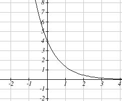
Example 1
x
Sketch a graph of f ( x
1
) =
4
3
This graph will have a vertical intercept at (0,4), and
pass through the point 4
,
1 . Since b < 1, the graph
3
will be decreasing towards zero. Since a > 0, the graph
will be concave up.
We can also see from the graph the long run behavior:
as x → ∞ , f ( x) → 0 and as x → −∞ , f ( x) → ∞ .
234 Chapter 4
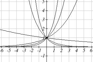
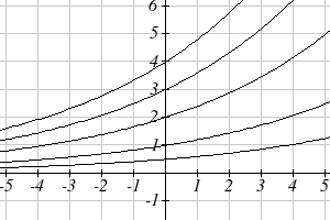
To get a better feeling for the effect of a and b on the graph, examine the sets of graphs
below. The first set shows various graphs, where a remains the same and we only change
the value for b.
x
(13)
3 x
2 x <