38.8
Utilizing the exponent property on the left,
1.0264
41.3
t log
log
=
1.0224
38.8
Dividing gives
41.3
log
38.8
t
=
≈15.991 years
1.0264
log
1.0224
Section 4.4 Logarithmic Properties 259
While the answer does not immediately appear identical to that produced using the
previous method, note that by using the difference property of logs, the answer could be
rewritten:
41.3
log
38.8
log(41.3) − log(38.8)
t =
=
1.0264 log(1.0264) − log(1.0224)
log1.0224
While both methods work equally well, it often requires fewer steps to utilize algebra
before taking logs, rather than relying solely on log properties.
Try it Now
3. Tank A contains 10 liters of water, and 35% of the water evaporates each week.
Tank B contains 30 liters of water, and 50% of the water evaporates each week. In how
many weeks will the tanks contain the same amount of water?
Important Topics of this Section
Inverse
Exponential
Change of base
Sum of logs property
Difference of logs property
Solving equations using log rules
Try it Now Answers
1. 5
2. 12
3. 4.1874 weeks
260 Chapter 4
Section 4.4 Exercises
Simplify to a single logarithm, using logarithm properties.
1. log 28 − log 7
2. log 32 − log 4
3 (
)
3 ( )
3 (
)
3 ( )
3.
1
log
−
4.
1
log
−
3 7
4 5
5.
1
log
+
log 50
6. log 3 + log (7)
4 ( )
3
3 (
)
10
4
7. 1 log 8
8. 1 log 36
5 (
)
7 ( )
3
2
9.
( 4 x)+ ( 5
log 2
log 3 x )
10. ( 2
x ) + ( 3
ln 4
ln 3 x )
11. ( 9
x ) − ( 2
ln 6
ln 3 x )
12.
( 4
log 12 x ) − log(4 x)
13. 2log( x) + 3log( x + )
1
14.
( x)+
( 2
3log
2log x )
15.
( x) 1
log
− log( y) + 3log( z)
16.
( x) 1
2log
+ log( y) − log( z)
2
3
Use logarithm properties to expand each expression.
15 13
2 3
17. log x y
18. log a b
19
z
5
c
2
−
2
−
3
19. ln a
20. ln a b
4
−
5
b c
5
c−
21.
( 3 4
log x y− )
22.
( 3− 2
log x y )
23. ln
y
x
y
24. ln
1 y
−
2
1− x
25. log( 2 3 3 2 5
x y x y )
26. log( 3 4 7 3 9
x y x y )
Section 4.4 Logarithmic Properties 261
Solve each equation for the variable.
27. 4 x−7
9 x−6
4
= 3
28. 2 x−5
3 x−7
2
= 7
29. 17(1.14) x 19(1.16) x
=
30. 20(1.07) x 8(1.13) x
=
31. 0.12 t
0.08
5
= 10
t
e
e
32. 0.09
0.14
3
t
t
e
= e
33. log 7 x + 6 = 3
34. log (2 x + 4) = 2
2 (
)
3
35. 2ln (3x) + 3 =1
36. 4ln (5 x) + 5 = 2
37.
( 3
log x ) = 2
38.
( 5
log x ) = 3
39. log( x) + log( x + 3) = 3
40. log( x + 4) + log( x) = 9
41. log( x + 4) − log( x + 3) =1
42. log( x + 5) − log( x + 2) = 2
43. log ( 2
x − log ( x +1) =1
44.
2
log ( x ) − log ( x + 2) = 5
6
)
6
3
3
45. log( x +12) = log( x) + log(12)
46. log( x +15) = log( x) + log(15)
47. ln ( x) + ln ( x − 3) = ln (7 x)
48. ln ( x) + ln ( x − 6) = ln (6 x)
262 Chapter 4
Section 4.5 Graphs of Logarithmic Functions
Recall that the exponential function
x
f ( x) = 2 produces this table of values
x
-3
-2
-1
0
1
2
3
f(x)
1
1
1
1
2
4
8
8
4
2
Since the logarithmic function is an inverse of the exponential, g( x)=log ( x) produces 2
the table of values
x
1
1
1
1
2
4
8
8
4
2
g(x)
-3
-2
-1
0
1
2
3
In this second table, notice that
1) As the input increases, the output increases.
2) As input increases, the output increases more slowly.
3) Since the exponential function only outputs positive values, the logarithm can
only accept positive values as inputs, so the domain of the log function is ( ,
0 ∞) .
4) Since the exponential function can accept all real numbers as inputs, the logarithm
can output any real number, so the range is all real numbers or (−∞,∞) .
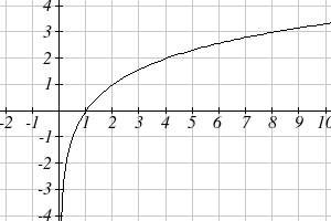
Sketching the graph, notice that as the input
approaches zero from the right, the output of
the function grows very large in the negative
direction, indicating a vertical asymptote at
x = 0.
In symbolic notation we write
as x → +
0 , f ( x) → −∞ , and
as x → ∞, f ( x) → ∞
Graphical Features of the Logarithm
Graphically, in the function g( x) = log x
b ( )
The graph has a horizontal intercept at (1, 0)
The graph has a vertical asymptote at x = 0
The graph is increasing and concave down
The domain of the function is x > 0, or ( ,
0 ∞)
The range of the function is all real numbers, or (−∞,∞)
When sketching a general logarithm with base b, it can be helpful to remember that the
graph will pass through the points (1, 0) and ( b, 1).
Section 4.5 Graphs of Logarithmic Functions 263
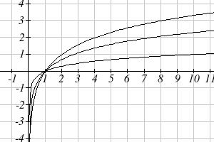
To get a feeling for how the base affects the shape of the graph, examine the graphs
below.
log ( x)
2
ln( x)
log( x)
Notice that the larger the base, the slower the graph grows. For example, the common
log graph, while it grows without bound, it does so very slowly. For example, to reach an
output of 8, the input must be 100,000,000.
Another important observation made was the domain of the logarithm. Like the
reciprocal and square root functions, the logarithm has a restricted domain which must be
considered when finding the domain of a composition involving a log.
Example 1
Find the domain of the function f ( x) = l 5
og( − 2 x)
The logarithm is only defined with the input is positive, so this function will only be
defined when 5 − 2 x > 0. Solving this inequality,
− 2 x > 5
−
5
x < 2
The domain of this function is
5
x < , or in interval notation,
5
− ∞,
2
2
Try it Now
1. Find the domain of the function f ( x) = log( x − )
5 + 2 ; before solving this as an
inequality, consider how the function has been transformed.
264 Chapter 4
Transformations of the Logarithmic Function
Transformations can be applied to a logarithmic function using the basic transformation
techniques, but as with exponential functions, several transformations result in interesting
relationships.
log c x
First recall the change of base property tells us that
1
log
=
=
log
b x
c x
log
log
c b
c b
From this, we can see that log
is a vertical stretch or compression of the graph of the
b x
log
graph. This tells us that a vertical stretch or compression is equivalent to a change
c x
of base. For this reason, we typically represent all graphs of logarithmic functions in
terms of the common or natural log functions.
Next, consider the effect of a horizontal compression on the graph of a logarithmic
function. Considering f ( x) = log( cx) , we can use the sum property to see
f ( x) = log( cx) = log( c) + log( x)
Since log( c) is a constant, the effect of a horizontal compression is the same as the effect
of a vertical shift.
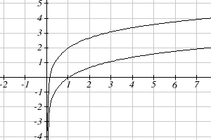
Example 2
Sketch f ( x) = ln( x) and g( x) = ln( x) + 2 .
Graphing these,
g( x) = ln( x) + 2
f ( x) = ln( x)
Note that, this vertical shift could also be written as a horizontal compression:
g( x) = ln( x) + 2 = ln( x) + ln( 2
e ) = ln( 2
e x) .
While a horizontal stretch or compression can be written as a vertical shift, a horizontal
reflection is unique and separate from vertical shifting.
Finally, we will consider the effect of a horizontal shift on the graph of a logarithm
Section 4.5 Graphs of Logarithmic Functions 265
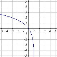
Example 3
Sketch a graph of f ( x) = ln( x + )
2 .
This is a horizontal shift to the left by 2 units. Notice that none of our logarithm rules
allow us rewrite this in another form, so the effect of this transformation is unique.
Shifting the graph,
Notice that due to the horizontal shift, the vertical asymptote shifted to x = -2, and the
domain shifted to ( 2,
− ∞).
Combining these transformations,
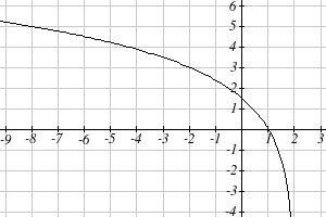
Example 4
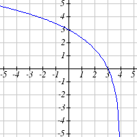
Sketch a graph of f ( x) = 5log(− x + 2).
Factoring the inside as f( x) =5log(−( x− ))2 reveals that this graph is that of the common logarithm, horizontally reflected, vertically stretched by a factor of 5, and
shifted to the right by 2 units.
The vertical asymptote will be shifted to
x = 2, and the graph will have domain
(∞,2) . A rough sketch can be created by
using the vertical asymptote along with a
couple points on the graph, such as
f )
1
( = 5log( 1
− + )
2 = 5log( )
1 = 0
f (− )
8 = 5log(−(− )
8 + 2) = 5log( )
10 = 5
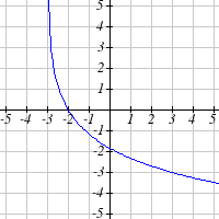
Try it Now
2. Sketch a graph of the function f ( x) = 3
− log( x − )
2 +1.
266 Chapter 4
Transformations of Logs
Any transformed logarithmic function can be written in the form
f ( x) = a log( x − b) + k , or f ( x) = a log(−( x − b)) + k if horizontally reflected, where
x = b is the vertical asymptote.
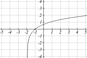
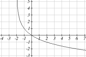
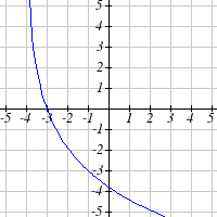
Example 5
Find an equation for the logarithmic function graphed below.
This graph has a vertical asymptote at x = –2 and has been vertically reflected. We do
not know yet the vertical shift (equivalent to horizontal stretch) or the vertical stretch
(equivalent to a change of base). We know so far that the equation will have form
f ( x) = − a log( x + )
2 + k
It appears the graph passes through the points (–1, 1) and (2, –1). Substituting in (–1, 1),
1 = − a log(−1+ )
2 + k
1 = − a log( )
1 + k
1 = k
Next, substituting in (2, –1),
−1 = − a log(2 + )
2 +1
− 2 = − a log(4)
2
a = log( )4
This gives us the equation
2
f ( x) = −
log( x + )
2 +1.
log( )
4
This could also be written as f ( x) = 2
− log ( x + 2) +1.
4
Flashback
3. Write the domain and range of the function graphed in Example 5, and describe its
long run behavior.
Section 4.5 Graphs of Logarithmic Functions 267
Important Topics of this Section
Graph of the logarithmic function (domain and range)
Transformation of logarithmic functions
Creating graphs from equations
Creating equations from graphs
Try it Now Answers
1. Domain: { x| x > 5}
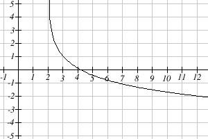
2.
Flashback Answers
3. Domain: { x| x>-2}, Range: all real numbers; As x → − +
2 , f ( x) → ∞ and as
x → ∞, f ( x) → −∞ .
268 Chapter 4
Section 4.5 Exercises
For each function, find the domain and the vertical asymptote.
1. f ( x) = log( x − 5)
2. f ( x) = log( x + 2)
3. f ( x) = ln (3− x)
4. f ( x) = ln (5 − x)
5. f ( x) = log(3 x + )
1
6. f ( x) = log(2 x + 5)
7. f ( x) = 3log(− x) + 2
8. f ( x) = 2log(−