Example 1
Describe all values, x, within a distance of 4 from the number 5.
We want the distance between x and 5 to be less than or equal to 4. The distance can be
represented using the absolute value, giving the expression
x − 5 ≤ 4
Example 2
A 2010 poll reported 78% of Americans believe that people who are gay should be able
to serve in the US military, with a reported margin of error of 3%9. The margin of error tells us how far off the actual value could be from the survey value10. Express the set of possible values using absolute values.
Since we want the size of the difference between the actual percentage, p, and the
reported percentage to be less than 3%,
p − 78 ≤ 3
9 http://www.pollingreport.com/civil.htm, retrieved August 4, 2010
10 Technically, margin of error usually means that the surveyors are 95% confident that actual value falls
within this range.
Section 2.5 Absolute Value Functions 147
Try it Now
1. Students who score within 20 points of 80 will pass the test. Write this as a distance
from 80 using the absolute value notation.
Important Features
The most significant feature of the absolute value graph is the corner point where the
graph changes direction. When finding the equation for a transformed absolute
value function, this point is very helpful for determining the horizontal and vertical
shifts.
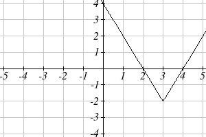
Example 3
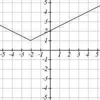
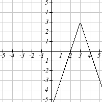
Write an equation for the function graphed below.
The basic absolute value function changes direction at the origin, so this graph has been
shifted to the right 3 and down 2 from the basic toolkit function. We might also notice
that the graph appears stretched, since the linear portions have slopes of 2 and -2. From
this information we can write the equation:
f ( x) = 2 x − 3 − 2 , treating the stretch as a vertical stretch
f ( x) = 2( x − )
3 − 2, treating the stretch as a horizontal compression
Note that these equations are algebraically equivalent – the stretch for an absolute value
function can be written interchangeably as a vertical or horizontal stretch/compression.
If you had not been able to determine the stretch based on the slopes of the lines, you
can solve for the stretch factor by putting in a known pair of values for x and f(x)
f ( x) = a x − 3 − 2
Now substituting in the point (1, 2)
2 = a 1− 3 − 2
4 = 2 a
a = 2
148 Chapter 2
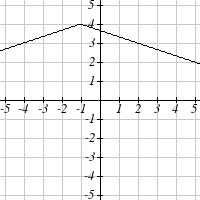
Try it Now
2. Given the description of the transformed absolute value function write the equation.
The absolute value function is horizontally shifted left 2 units, is vertically flipped, and
vertically shifted up 3 units,
The graph of an absolute value function will have a vertical intercept when the input
is zero. The graph may or may not have horizontal intercepts, depending on how the
graph has been shifted and reflected. It is possible for the absolute value function to
have zero, one, or two horizontal intercepts.
Zero horizontal intercepts
One
Two
To find the horizontal intercepts, we will need to solve an equation involving an
absolute value.
Notice that the absolute value function is not one-to-one, so typically inverses of
absolute value functions are not discussed.
Solving Absolute Value Equations
To solve an equation like 8= 2 x−6 , we can notice that the absolute value will be
equal to eight if the quantity inside the absolute value were 8 or -8. This leads to
two different equations we can solve independently:
2 x − 6 = 8
or
2 x − 6 = 8
−
2 x = 14
2 x = 2
−
x = 7
x = 1
−
Solutions to Absolute Value Equations
An equation of the form A = B , with B ≥ 0 , will have solutions when
A = B or A = − B
Section 2.5 Absolute Value Functions 149
Example 4
Find the horizontal intercepts of the graph of f ( x) = 4 x +1 − 7
The horizontal intercepts will occur when f( x) =0. Solving,
0 = 4 x +1 − 7
Isolate the absolute value on one side of the equation
7 = 4 x +1
Now we can break this into two separate equations:
7 = 4 x +1
− 7 = 4 x +1
6 = 4 x
or
− 8 = 4 x
6 3
x
−
= =
8
x =
= 2
−
4 2
4
The graph has two horizontal intercepts, at
3
x = and x = -2
2
Example 5
Solve 1 = 4 x − 2 + 2
Isolating the absolute value on one side the equation,
1 = 4 x − 2 + 2
−1 = 4 x − 2
1
− = x − 2
4
At this point, we notice that this equation has no solutions – the absolute value always
returns a positive value, so it is impossible for the absolute value to equal a negative
value.
Try it Now
3. Find the horizontal & vertical intercepts for the function f ( x) = − x + 2 + 3
Solving Absolute Value Inequalities
When absolute value inequalities are written to describe a set of values, like the
inequality x − 5 ≤ 4 we wrote earlier, it is sometimes desirable to express this set of
values without the absolute value, either using inequalities, or using interval
notation.
150 Chapter 2
We will explore two approaches to solving absolute value inequalities:
1) Using the graph
2) Using test values
Example 6
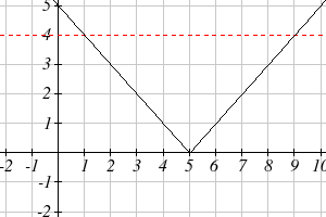
Solve x − 5 ≤ 4
With both approaches, we will need to know first where the corresponding equality is
true. In this case we first will find where x − 5 = 4 . We do this because the absolute
value is a nice friendly function with no breaks, so the only way the function values can
switch from being less than 4 to being greater than 4 is by passing through where the
values equal 4. Solve x − 5 = 4 ,
x − 5 = 4
x − 5 = 4
−
or
x = 9
x = 1
To use a graph, we can sketch the function f ( x) = x − 5 . To help us see where the outputs are 4, the line g( x) = 4 could also be sketched.
On the graph, we can see that indeed the output values of the absolute value are equal to
4 at x = 1 and x = 9. Based on the shape of the graph, we can determine the absolute
value is less than or equal to 4 between these two points, when 1 ≤ x ≤ 9. In interval
notation, this would be the interval [1,9].
As an alternative to graphing, after determining that the absolute value is equal to 4 at x
= 1 and x = 9, we know the graph can only change from being less than 4 to greater than
4 at these values. This divides the number line up into three intervals: x<1, 1< x<9, and
x>9. To determine when the function is less than 4, we could pick a value in each
interval and see if the output is less than or greater than 4.
Section 2.5 Absolute Value Functions 151
Interval
Test x
f(x)
<4 or >4?
x<1
0
0 − 5 = 5
greater
1< x<9
6
6 − 5 = 1
less
x>9
11
11− 5 = 6
greater
Since 1≤ x ≤9 is the only interval in which the output at the test value is less than 4,
we can conclude the solution to x − 5 ≤ 4 is 1 ≤ x ≤ 9.
Example 7
Given the function
1
f ( x) = − 4 x − 5 + 3, determine for what x values the function
2
values are negative.
We are trying to determine where f(x) < 0, which is when 1
− 4 x − 5 + 3 < 0 . We begin
2
by isolating the absolute value:
1
− 4 x − 5 < 3
−
when we multiply both sides by -2, it reverses the inequality
2
4 x − 5 > 6
Next we solve for the equality 4 x − 5 = 6
4 x − 5 = 6
4 x − 5 = 6
−
4 x = 11 or
4 x = 1
−
11
x
−
=
1
x =
4
4
We can now either pick test values or sketch a graph of the function to determine on
which intervals the original function value are negative. Notice that it is not even really
important exactly what the graph looks like, as long as we know that it crosses the
−
horizontal axis at
1
x =
and
11
x =
, and that the graph has been reflected vertically.
4
4
152 Chapter 2
From the graph of the function, we can see the function values are negative to the left of
−
the first horizontal intercept at
1
x =
, and negative to the right of the second intercept
4
at
11
x =
. This gives us the solution to the inequality:
4
−1
11
x <
or x >
4
4
In interval notation, this would be
−1 11
− ∞,
∪ ,∞
4 4
Try it Now
4. Solve − 2 k − 4 ≤ 6
−
Important Topics of this Section
The properties of the absolute value function
Solving absolute value equations
Finding intercepts
Solving absolute value inequalities
Try it Now Answers
1. Using the variable p, for passing, p − 80 ≤ 20
2. f ( x) = − x + 2 + 3
3. f(0) = 1, so the vertical intercept is at (0,1). f(x)= 0 when x = -5 and x = 1 so the horizontal intercepts are at (-5,0) & (1,0)
4. k < 1or k > 7 ; in interval notation this would be (− ∞ )
1, ∪ ( ,
7 ∞)
Section 2.5 Absolute Value Functions 153
Section 2.5 Exercises
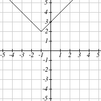
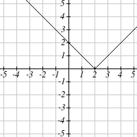
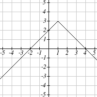
Write an equation for each transformation of f( x) |= x|
1.
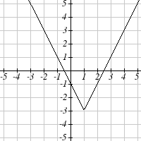
2.
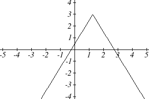
3.
4.
Sketch a graph of each function
5. f ( x)
= − | x −1| 1
−
6. f ( x) =
− x + 3 + 4
7. f ( x) = 2 x + 3 +1
8. f ( x) = 3 x − 2 − 3
9. f ( x) = 2 x − 4 − 3
10. f ( x) = 3 x + 9 + 2
Solve each the equation
11. | 5 x − 2 |=11
12. | 4 x + 2 |=15
13. 2 | 4 − x |= 7
14. 3| 5 − x |= 5
15. 3 x +1 − 4 = 2
−
16. 5 x − 4 − 7 = 2
154 Chapter 2
Find the horizontal and vertical intercepts of each function
17. f ( x) = 2 | x +1| 10
−
18. f ( x) = 4 x − 3 + 4
19. f ( x) = 3
− x − 2 −1
20. f ( x) = 2
− x +1 + 6
Solve each inequality
21. | x + 5 |< 6
22. | x − 3 |< 7
23. | x − 2 |≥ 3
24. | x + 4 |≥ 2
25. | 3 x + 9 | < 4
26. | 2 x − 9 | ≤ 8
3.1 Power and Polynomial Functions 155
Chapter 3: Polynomial and Rational Functions
Section 3.1 Power Functions & Polynomial Functions
A square is cut out of cardboard, with each side having length L. If we wanted to write a
function for the area of the square, with L as the input and the area as output, you may
recall that the area of a rectangle can be found by multiplying the length times the width.
Since our shape is a square, the length & the width are the same, giving the formula:
2
(
A L) = L ⋅ L = L
Likewise, if we wanted a function for the volume of a cube with each side having some
length L, you may recall volume of a rectangular box can be found by multiplying length
by width by height, which are all equal for a cube, giving the formula:
3
V ( L) = L ⋅ L ⋅ L = L
These two functions are examples of power functions, functions that are some power of
the variable.
Power Function
A power function is a function that can be represented in the form
p
f ( x) = x
Where the base is a variable and the exponent, p, is a number.
Example 1
Which of our toolkit functions are power functions?
The constant and identity functions are power functions, since they can be written as
0
f ( x) = x and
1
f ( x) = x respectively.
The quadratic and cubic functions are both power functions with whole number powers:
2
f ( x) = x and
3
f ( x) = x .
The reciprocal and reciprocal squared functions are both power functions with negative
whole number powers since they can be written as
1
f ( x)
−
= x and
2
f ( x)
−
= x .
The square and cube root functions are both power functions with fractional powers
since they can be written as
1 2
f ( x) = x or
1 3
f ( x) = x .
This chapter is part of Precalculus: An Investigation of Functions © Lippman & Rasmussen 2011.
This material is licensed under a Creative Commons CC-BY-SA license.
156 Chapter 3
Try it Now
1. What point(s) do the toolkit power functions have in common?
6
f
4
( x) = x
f ( x) = x
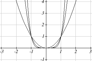
Characteristics of Power Functions
Shown to the right are the graphs of
2
f ( x) = x
2
4
6
f ( x) = x , f ( x) = x , and f ( x) = x , all even whole number powers. Notice that all
these graphs have a fairly similar shape, very
similar to the quadratic toolkit, but as the
power increases the graphs flatten somewhat
near the origin, and become steeper away
from the origin.
To describe the behavior as numbers become larger and larger, we use the idea of
infinity. The symbol for positive infinity is ∞ , and − ∞ for negative infinity. When we
say that “x approaches infinity”, which can be symbolically written as x → ∞ , we are
describing a behavior – we are saying that x is getting large in the positive direction.
With the even power function, as the input becomes large in either the positive or
negative direction, the output values become very large positive numbers. Equivalently,
we could describe this by saying that as x approaches positive or negative infinity, the f(x)
values approach positive infinity. In symbolic form, we could write: as x → ±∞ ,
f ( x) → ∞ .
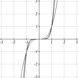
5
f ( x) = x
7
f ( x) = x
Shown here are the graphs of
3
5
7
f ( x) =