2013/02/11 14:28:20 -0600
Up to this point in the book, we have developed the basic two-band wavelet system in some detail, trying to provide insight and intuition into this new mathematical tool. We will now develop a variety of interesting and valuable generalizations and extensions to the basic system, but in much less detail. We hope the detail of the earlier part of the book can be transferred to these generalizations and, together with the references, will provide an introduction to the topics.
A qualitative descriptive presentation of the decomposition of a signal using wavelet systems or wavelet transforms consists of partitioning the time–scale plane into tiles according to the indices k and j defined in Equation 2.5. That is possible for orthogonal bases (or tight frames) because of Parseval's theorem. Indeed, it is Parseval's theorem that states that the signal energy can be partitioned on the time-scale plane. The shape and location of the tiles shows the logarithmic nature of the partitioning using basic wavelets and how the M-band systems or wavelet packets modify the basic picture. It also allows showing that the effects of time- or shift-varying wavelet systems, together with M-band and packets, can give an almost arbitrary partitioning of the plane.
The energy in a signal is given in terms of the DWT by Parseval's relation in Equation 3.36 or Equation 5.24. This shows the energy is a function of the translation index k and the scale index j.

The wavelet transform allows analysis of a signal or parameterization of a signal that can locate energy in both the time and scale (or frequency) domain within the constraints of the uncertainty principle. The spectrogram used in speech analysis is an example of using the short-time Fourier transform to describe speech simultaneously in the time and frequency domains.
This graphical or visual description of the partitioning of energy in a signal using tiling depends on the structure of the system, not the parameters of the system. In other words, the tiling partitioning will depend on whether one uses M=2 or M=3, whether one uses wavelet packets or time-varying wavelets, or whether one uses over-complete frame systems. It does not depend on the particular coefficients h(n) or hi(n), on the number of coefficients N, or the number of zero moments. One should remember that the tiling may look as if the indices j and k are continuous variables, but they are not. The energy is really a function of discrete variables in the DWT domain, and the boundaries of the tiles are symbolic of the partitioning. These tiling boundaries become more literal when the continuous wavelet transform (CWT) is used as described in Section 8.8, but even there it does not mean that the partitioned energy is literally confined to the tiles.
In many applications, one studies the decomposition of a signal in terms of basis functions. For example, stationary signals are decomposed into the Fourier basis using the Fourier transform. For nonstationary signals (i.e., signals whose frequency characteristics are time-varying like music, speech, images, etc.) the Fourier basis is ill-suited because of the poor time-localization. The classical solution to this problem is to use the short-time (or windowed) Fourier transform (STFT). However, the STFT has several problems, the most severe being the fixed time-frequency resolution of the basis functions. Wavelet techniques give a new class of (potentially signal dependent) bases that have desired time-frequency resolution properties. The “optimal” decomposition depends on the signal (or class of signals) studied. All classical time-frequency decompositions like the Discrete STFT (DSTFT), however, are signal independent. Each function in a basis can be considered schematically as a tile in the time-frequency plane, where most of its energy is concentrated. Orthonormality of the basis functions can be schematically captured by nonoverlapping tiles. With this assumption, the time-frequency tiles for the standard basis (i.e., delta basis) and the Fourier basis (i.e., sinusoidal basis) are shown in Figure 8.1.
The DSTFT basis functions are of the form

where w(t) is a window function
40. If these functions form an orthogonal (orthonormal) basis, x(t)=∑j,k〈x , wj,k〉wj,k(t). The DSTFT coefficients,
〈x , wj,k〉, estimate the presence of signal components centered at
 in the time-frequency plane, i.e., the DSTFT gives a uniform
tiling of the time-frequency plane with the basis functions {wj,k (t)}.
If Δt and Δω are time and frequency resolutions
respectively of w(t), then the uncertainty principle demands that
ΔtΔω≤1/229, 123. Moreover,
if the basis is orthonormal, the Balian-Low theorem implies either
Δt or Δω is infinite.
Both Δt and Δω can be controlled by the choice of
w(t), but for any particular choice, there will be signals for which
either the time or frequency resolution is not adequate.
Figure 8.1 shows the
time-frequency tiles associated with the STFT basis for a narrow and wide
window, illustrating the inherent time-frequency trade-offs
associated with this basis. Notice that the tiling schematic holds for
several choices of windows (i.e., each figure represents all DSTFT
bases with the particular time-frequency resolution
characteristic).
in the time-frequency plane, i.e., the DSTFT gives a uniform
tiling of the time-frequency plane with the basis functions {wj,k (t)}.
If Δt and Δω are time and frequency resolutions
respectively of w(t), then the uncertainty principle demands that
ΔtΔω≤1/229, 123. Moreover,
if the basis is orthonormal, the Balian-Low theorem implies either
Δt or Δω is infinite.
Both Δt and Δω can be controlled by the choice of
w(t), but for any particular choice, there will be signals for which
either the time or frequency resolution is not adequate.
Figure 8.1 shows the
time-frequency tiles associated with the STFT basis for a narrow and wide
window, illustrating the inherent time-frequency trade-offs
associated with this basis. Notice that the tiling schematic holds for
several choices of windows (i.e., each figure represents all DSTFT
bases with the particular time-frequency resolution
characteristic).
The discrete wavelet transform (DWT) is another signal-independent tiling
of the time-frequency plane suited for signals where high frequency signal components
have shorter duration than low frequency signal components. Time-frequency
atoms for the DWT,  ,
are obtained by translates and scales of the wavelet function ψ(t).
One shrinks/stretches the wavelet to capture high-/low-frequency components
of the signal. If these atoms form an orthonormal basis, then x(t)=∑j,k〈x , ψj,k〉ψj,k(t). The DWT coefficients,
〈x , ψj,k〉, are a measure of the energy of the signal components
located at
,
are obtained by translates and scales of the wavelet function ψ(t).
One shrinks/stretches the wavelet to capture high-/low-frequency components
of the signal. If these atoms form an orthonormal basis, then x(t)=∑j,k〈x , ψj,k〉ψj,k(t). The DWT coefficients,
〈x , ψj,k〉, are a measure of the energy of the signal components
located at  in the time-frequency plane, giving yet another
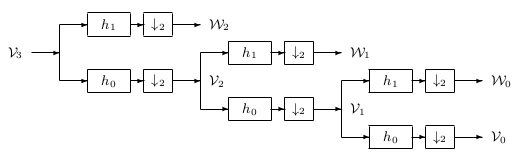
tiling of the time-frequency plane. As discussed in Chapter: Filter Banks and the Discrete Wavelet Transform and Chapter: Filter Banks and Transmultiplexers,
the DWT (for compactly supported wavelets) can be efficiently computed
using two-channel unitary FIR filter banks 27.
Figure 8.3 shows the corresponding
tiling description which illustrates time-frequency resolution properties
of a DWT basis.
If you look along the frequency (or scale) axis at some
particular time (translation), you can imagine seeing the frequency
response of the filter bank as shown in Equation 8.7 with the
logarithmic bandwidth of each channel. Indeed, each horizontal strip in
the tiling of Figure 8.3 corresponds to each channel, which
in turn corresponds to a scale j. The location of the tiles
corresponding to each coefficient is shown in Figure 8.4.
If at a particular scale, you imagine the translations along the k axis,
you see the construction of the components of a signal at that scale. This
makes it obvious that at lower resolutions (smaller j) the translations
are large and at higher resolutions the translations are small.
in the time-frequency plane, giving yet another
tiling of the time-frequency plane. As discussed in Chapter: Filter Banks and the Discrete Wavelet Transform and Chapter: Filter Banks and Transmultiplexers,
the DWT (for compactly supported wavelets) can be efficiently computed
using two-channel unitary FIR filter banks 27.
Figure 8.3 shows the corresponding
tiling description which illustrates time-frequency resolution properties
of a DWT basis.
If you look along the frequency (or scale) axis at some
particular time (translation), you can imagine seeing the frequency
response of the filter bank as shown in Equation 8.7 with the
logarithmic bandwidth of each channel. Indeed, each horizontal strip in
the tiling of Figure 8.3 corresponds to each channel, which
in turn corresponds to a scale j. The location of the tiles
corresponding to each coefficient is shown in Figure 8.4.
If at a particular scale, you imagine the translations along the k axis,
you see the construction of the components of a signal at that scale. This
makes it obvious that at lower resolutions (smaller j) the translations
are large and at higher resolutions the translations are small.
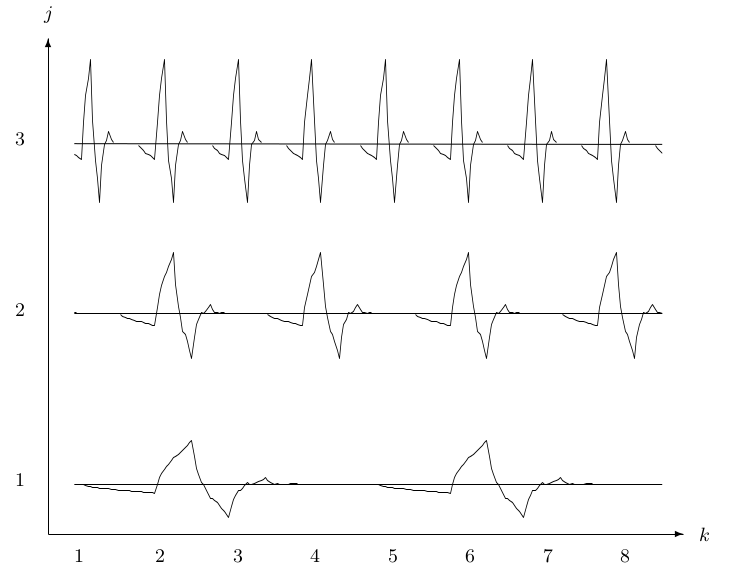
The tiling of the time-frequency plane is a powerful graphical method for understanding the properties of the DWT and for analyzing signals. For example, if the signal being analyzed were a single wavelet itself, of the form

the DWT would have only one nonzero coefficient, d2(2). To see that the DWT is not time (or shift) invariant, imagine shifting f(t) some noninteger amount and you see the DWT changes considerably. If the shift is some integer, the energy stays the same in each scale, but it “spreads out" along more values of k and spreads differently in each scale. If the shift is not an integer, the energy spreads in both j and k. There is no such thing as a “scale limited" signal corresponding to a band-limited (Fourier) signal if arbitrary shifting is allowed. For integer shifts, there is a corresponding concept 53.
Notice that for general, nonstationary signal analysis, one desires methods for controlling the tiling of the time-frequency plane, not just using the two special cases above (their importance notwithstanding). An alternative way to obtain orthonormal wavelets ψ(t) is using unitary FIR filter bank (FB) theory. That will be done with M-band DWTs, wavelet packets, and time-varying wavelet transforms addressed in Section: Multiplicity-M (M-Band) Scaling Functions and Wavelets and Section: Wavelet Packets and Chapter: Filter Banks and Transmultiplexers respectively.
Remember that the tiles represent the relative size of the translations and scale change. They do not literally mean the partitioned energy is confined to the tiles. Representations with similar tilings can have very different characteristics.
While the use of a scale multiplier M of two in Equation 6.1 or Equation 8.4 fits many problems, coincides with the concept of an octave, gives a binary tree for the Mallat fast algorithm, and gives the constant-Q or logarithmic frequency bandwidths, the conditions given in Chapter: The Scaling Function and Scaling Coefficients, Wavelet and Wavelet Coefficients and Section: Further Properties of the Scaling Function and Wavelet can be stated and proved in a more general setting where the basic scaling equation 148, 147, 43, 121, 59, 52, 136 rather than the specific doubling value of M=2. Part of the motivation for a larger M comes from a desire to have a more flexible tiling of the time-scale plane than that resulting from the M=2 wavelet or the short-time Fourier transform discussed in Section: Tiling the Time–Frequency or Time–Scale Plane. It also comes from a desire for some regions of uniform band widths rather than the logarithmic spacing of the frequency responses illustrated in Figure: Frequency Bands for the Analysis Tree. The motivation for larger M also comes from filter bank theory which is discussed in Chapter: Filter Banks and Transmultiplexers.
We pose the more general multiresolution formulation where Equation 6.1 becomes

In some cases, M may be allowed to be a rational number; however, in most cases it must be an integer, and in Equation 6.1 it is required to be 2. In the frequency domain, this relationship becomes

and the limit after iteration is

assuming the product converges and Φ(0) is well defined. This is a generalization of Equation 6.52 and is derived in Equation 6.74.
These theorems, relationships, and properties are generalizations of those
given in Chapter: The Scaling Function and Scaling Coefficients, Wavelet and Wavelet Coefficients and Section: Further Properties of the Scaling Function and Wavelet with some outline proofs or
derivations given in the Appendix. For the multiplicity-M problem, if the
support of the scaling function and wavelets and their respective coefficients
is finite and the system is
orthogonal or a tight frame, the length of the scaling function vector or
filter h(n) is a multiple of the multiplier M. This is  , where
Resnikoff and Wells 119 call M the rank of the system and G the
genus.
, where
Resnikoff and Wells 119 call M the rank of the system and G the
genus.
The results of Equation 6.10, Equation 6.14, Equation 6.16, and Equation 6.17 become
Theorem 28 If φ(t) is an L1 solution to Equation 8.4 and
 , then

This is a generalization of the basic multiplicity-2 result in Equation 6.10 and does not depend on any particular normalization or orthogonality of φ(t).
Theorem 29 If integer translates of the solution to Equation 8.4 are orthogonal, then

This is a generalization of Equation 6.14 and also does not depend on any normalization. An interesting corollary of this theorem is