2013/02/11 15:07:48 -0600
This chapter gives a brief discussion of several areas of application. It is intended to show what areas and what tools are being developed and to give some references to books, articles, and conference papers where the topics can be further pursued. In other words, it is a sort of annotated bibliography that does not pretend to be complete. Indeed, it is impossible to be complete or up-to-date in such a rapidly developing new area and in an introductory book.
In this chapter, we briefly consider the application of wavelet systems from two perspectives. First, we look at wavelets as a tool for denoising and compressing a wide variety of signals. Second, we very briefly list several problems where the application of these tools shows promise or has already achieved significant success. References will be given to guide the reader to the details of these applications, which are beyond the scope of this book.
To accomplish frequency domain signal processing, one can take the Fourier transform (or Fourier series or DFT) of a signal, multiply some of the Fourier coefficients by zero (or some other constant), then take the inverse Fourier transform. It is possible to completely remove certain components of a signal while leaving others completely unchanged. The same can be done by using wavelet transforms to achieve wavelet-based, wavelet domain signal processing, or filtering. Indeed, it is sometimes possible to remove or separate parts of a signal that overlap in both time and frequency using wavelets, something impossible to do with conventional Fourier-based techniques.
The classical paradigm for transform-based signal processing is illustrated in Figure 11.1 where the center “box" could be either a linear or nonlinear operation. The “dynamics" of the processing are all contained in the transform and inverse transform operation, which are linear. The transform-domain processing operation has no dynamics; it is an algebraic operation. By dynamics, we mean that a process depends on the present and past, and by algebraic, we mean it depends only on the present. An FIR (finite impulse response) filter such as is part of a filter bank is dynamic. Each output depends on the current and a finite number of past inputs (see Equation 4.11). The process of operating point-wise on the DWT of a signal is static or algebraic. It does not depend on the past (or future) values, only the present. This structure, which separates the linear, dynamic parts from the nonlinear static parts of the processing, allows practical and theoretical results that are impossible or very difficult using a completely general nonlinear dynamic system.
Linear wavelet-based signal processing consists of the processor block in Figure 11.1 multiplying the DWT of the signal by some set of constants (perhaps by zero). If undesired signals or noise can be separated from the desired signal in the wavelet transform domain, they can be removed by multiplying their coefficients by zero. This allows a more powerful and flexible processing or filtering than can be achieved using Fourier transforms. The result of this total process is a linear, time-varying processing that is far more versatile than linear, time-invariant processing. The next section gives an example of using the concentrating properties of the DWT to allow a faster calculation of the FFT.
In this section, we give an example of wavelet domain signal processing. Rather than computing the DFT from the time domain signal using the FFT algorithm, we will first transform the signal into the wavelet domain, then calculate the FFT, and finally go back to the signal domain which is now the Fourier domain.
Most methods of approximately calculating the discrete Fourier transform (DFT) involve calculating only a few output points (pruning), using a small number of bits to represent the various calculations, or approximating the kernel, perhaps by using cordic methods. Here we use the characteristics of the signal being transformed to reduce the amount of arithmetic. Since the wavelet transform concentrates the energy of many classes of signals onto a small number of wavelet coefficients, this can be used to improve the efficiency of the DFT 44, 48, 55, 43 and convolution 45.
The DFT is probably the most important
computational tool in signal processing. Because of the characteristics of
the basis functions, the DFT has
enormous capacity for the improvement of its arithmetic efficiency
15.
The classical Cooley-Tukey fast Fourier transform (FFT) algorithm has the
complexity of  .
Thus the Fourier transform and its fast algorithm, the FFT, are widely
used in many areas, including signal processing and numerical analysis.
Any scheme to speed up the FFT would be very desirable.
.
Thus the Fourier transform and its fast algorithm, the FFT, are widely
used in many areas, including signal processing and numerical analysis.
Any scheme to speed up the FFT would be very desirable.
Although the FFT has been studied extensively, there are still some desired properties that are not provided by the classical FFT. Here are some of the disadvantages of the FFT algorithm:
Pruning is not easy. When the number of input points or output points are small compared to the length of the DWT, a special technique called pruning 90 is often used. However, this often requires that the nonzero input data are grouped together. Classical FFT pruning algorithms do not work well when the few nonzero inputs are randomly located. In other words, a sparse signal may not necessarily give rise to faster algorithm.
No speed versus accuracy tradeoff. It is common to have a situation where some error would be allowed if there could be a significant increase in speed. However, this is not easy with the classical FFT algorithm. One of the main reasons is that the twiddle factors in the butterfly operations are unit magnitude complex numbers. So all parts of the FFT structure are of equal importance. It is hard to decide which part of the FFT structure to omit when error is allowed and the speed is crucial. In other words, the FFT is a single speed and single accuracy algorithm.
No built-in noise reduction capacity. Many real world signals are noisy. What people are really interested in are the DFT of the signals without the noise. The classical FFT algorithm does not have built-in noise reduction capacity. Even if other denoising algorithms are used, the FFT requires the same computational complexity on the denoised signal. Due to the above mentioned shortcomings, the fact that the signal has been denoised cannot be easily used to speed up the FFT.
The discrete Fourier transform (DFT) is defined for a length-N complex data sequence by

where we use  .
There are several ways to derive the different fast Fourier transform (FFT)
algorithms. It can be done by using index mapping 15, by
matrix factorization, or by polynomial factorization. In this chapter, we
only discuss the matrix factorization approach, and only discuss the so-called
radix-2 decimation in time (DIT) variant of the FFT.
.
There are several ways to derive the different fast Fourier transform (FFT)
algorithms. It can be done by using index mapping 15, by
matrix factorization, or by polynomial factorization. In this chapter, we
only discuss the matrix factorization approach, and only discuss the so-called
radix-2 decimation in time (DIT) variant of the FFT.
Instead of repeating the derivation of the FFT algorithm, we show the block diagram and matrix factorization, in an effort to highlight the basic idea and gain some insight. The block diagram of the last stage of a length-8 radix-2 DIT FFT is shown in Figure 11.2. First, the input data are separated into even and odd groups. Then, each group goes through a length-4 DFT block. Finally, butterfly operations are used to combine the shorter DFTs into longer DFTs.
The details of the butterfly operations are shown in Figure 11.3, where WNi=e–j2πi/N is called the twiddle factor. All the twiddle factors are of magnitude one on the unit circle. This is the main reason that there is no complexity versus accuracy tradeoff for the classical FFT. Suppose some of the twiddle factors had very small magnitude, then the corresponding branches of the butterfly operations could be dropped (pruned) to reduce complexity while minimizing the error to be introduced. Of course the error also depends on the value of the data to be multiplied with the twiddle factors. When the value of the data is unknown, the best way is to cutoff the branches with small twiddle factors.
The computational complexity of the FFT algorithm can be easily established. If we let CFFT(N) be the complexity for a length-N FFT, we can show
where O(N) denotes linear complexity. The solution to Equation Equation 11.2 is well known:

This is a classical case where the divide and conquer approach results in very effective solution.
The matrix point of view gives us additional insight. Let FN be
the  DFT matrix; i.e., FN(m,n)=e–j2πmn/N,
where
DFT matrix; i.e., FN(m,n)=e–j2πmn/N,
where  . Let SN be
the
. Let SN be
the  even-odd separation matrix; e.g.,

Clearly SN'SN=IN, where IN is the
 identity matrix. Then the DIT FFT is based on the following matrix
factorization,
identity matrix. Then the DIT FFT is based on the following matrix
factorization,

where TN/2 is a diagonal matrix with WNi,
 on the diagonal. We can visualize the
above factorization as
on the diagonal. We can visualize the
above factorization as
where we image the real part of DFT matrices, and the magnitude of the matrices for butterfly operations and even-odd separations. N is taken to be 128 here.
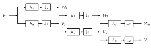
In this section, we briefly review the fundamentals of the discrete wavelet transform and introduce the necessary notation for future sections. The details of the DWT have been covered in other chapters.
At the heart of the discrete wavelet transform are a pair of filters h and g — lowpass and highpass respectively. They have to satisfy a set of constraints Figure: Sinc Scaling Function and Wavelet 110, 99, 108. The block diagram of the DWT is shown in Figure 11.4. The input data are first filtered by h and g then downsampled. The same building block is further iterated on the lowpass outputs.
The computational complexity of the DWT algorithm can also be easily established. Let CDWT(N) be the complexity for a length-N DWT. Since after each scale, we only further operate on half of the output data, we can show
which gives rise to the solution
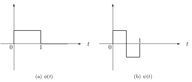
The operation in Figure 11.4 can also be expressed in matrix form WN; e.g., for Haar wavelet,

The orthogonality conditions on h and g ensure WN'WN=IN. The matrix for multiscale DWT is formed by WN for different N; e.g., for three scale DWT,

We could further iterate the building block on some of the highpass outputs. This generalization is called the wavelet packets 25.
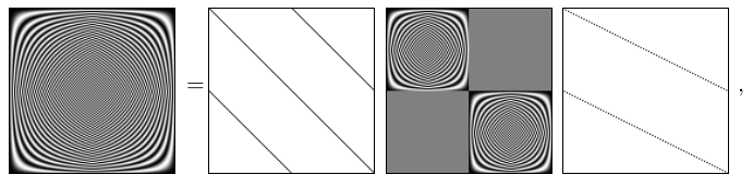
The key to the fast Fourier transform is the factorization of FN into several sparse matrices, and one of the sparse matrices represents two DFTs of half the length. In a manner similar to the DIT FFT, the following matrix factorization can be made:

where AN/2,BN/2,CN/2, and DN/2 are all diagonal matrices. The values on the diagonal of AN/2 and CN/2 are the length-N DFT (i.e., frequency response) of h, and the values on the diagonal of BN/2 and DN/2 are the length-N DFT of g. We can visualize the above factorization as
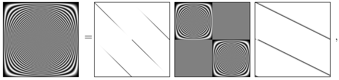
where we image the real part of DFT matrices, and the magnitude of the matrices for butterfly operations and the one-scale DWT using length-16 Daubechies' wavelets 26, 27. Clearly we can see that the new twiddle factors have non-unit magnitudes.
The above factorization suggests a DWT-based FFT algorithm. The block diagram of the last stage of a length-8 algorithm is shown in Figure 11.5. This scheme is iteratively applied to shorter length DFTs to get the full DWT based FFT algorithm. The final system is equivalent to a full binary tree wavelet packet transform 24 followe