2013/02/11 14:28:05 -0600
This chapter will provide an overview of the topics to be developed in the book. Its purpose is to present the ideas, goals, and outline of properties for an understanding of and ability to use wavelets and wavelet transforms. The details and more careful definitions are given later in the book.
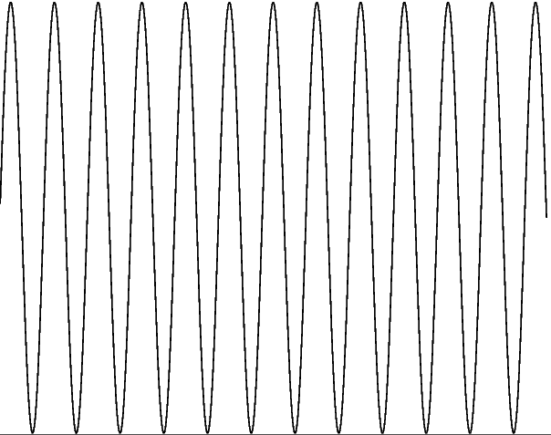
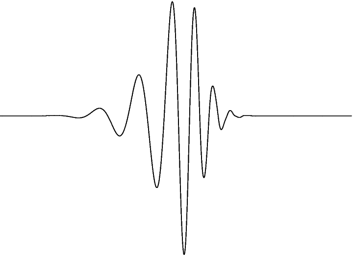
A wave is usually defined as an oscillating function of time or space, such as a sinusoid. Fourier analysis is wave analysis. It expands signals or functions in terms of sinusoids (or, equivalently, complex exponentials) which has proven to be extremely valuable in mathematics, science, and engineering, especially for periodic, time-invariant, or stationary phenomena. A wavelet is a “small wave", which has its energy concentrated in time to give a tool for the analysis of transient, nonstationary, or time-varying phenomena. It still has the oscillating wave-like characteristic but also has the ability to allow simultaneous time and frequency analysis with a flexible mathematical foundation. This is illustrated in Figure 2.1 with the wave (sinusoid) oscillating with equal amplitude over –∞≤t≤∞ and, therefore, having infinite energy and with the wavelet having its finite energy concentrated around a point.
We will take wavelets and use them in a series expansion of signals or functions much the same way a Fourier series uses the wave or sinusoid to represent a signal or function. The signals are functions of a continuous variable, which often represents time or distance. From this series expansion, we will develop a discrete-time version similar to the discrete Fourier transform where the signal is represented by a string of numbers where the numbers may be samples of a signal, samples of another string of numbers, or inner products of a signal with some expansion set. Finally, we will briefly describe the continuous wavelet transform where both the signal and the transform are functions of continuous variables. This is analogous to the Fourier transform.
Before delving into the details of wavelets and their properties, we need to get some idea of their general characteristics and what we are going to do with them 11.
A signal or function f(t) can often be better analyzed, described, or processed if expressed as a linear decomposition by

where ℓ is an integer index for the finite or infinite sum, aℓ are the real-valued expansion coefficients, and ψℓ(t) are a set of real-valued functions of t called the expansion set. If the expansion Equation 2.1 is unique, the set is called a basis for the class of functions that can be so expressed. If the basis is orthogonal, meaning

then the coefficients can be calculated by the inner product

One can see that substituting Equation 2.1 into Equation 2.3 and using Equation 2.2
gives the single ak coefficient. If the basis set is not orthogonal,
then a dual basis set  exists such that using Equation 2.3
with the dual basis gives the desired coefficients. This will be developed
in Chapter: A multiresolution formulation of Wavelet Systems.
exists such that using Equation 2.3
with the dual basis gives the desired coefficients. This will be developed
in Chapter: A multiresolution formulation of Wavelet Systems.
For a Fourier series, the orthogonal basis functions ψk(t) are
 and
and  with frequencies of kω0.
For a Taylor's
series, the nonorthogonal basis functions are simple monomials tk, and
for many other expansions they are various polynomials. There are
expansions that use splines and even fractals.
with frequencies of kω0.
For a Taylor's
series, the nonorthogonal basis functions are simple monomials tk, and
for many other expansions they are various polynomials. There are
expansions that use splines and even fractals.
For the wavelet expansion, a two-parameter system is constructed such that Equation 2.1 becomes

where both j and k are integer indices and the ψj,k(t) are the wavelet expansion functions that usually form an orthogonal basis.
The set of expansion coefficients aj,k are called the discrete wavelet transform (DWT) of f(t) and Equation 2.4 is the inverse transform.
The wavelet expansion set is not unique. There are many different wavelets systems that can be used effectively, but all seem to have the following three general characteristics 11.
A wavelet system is a set of building blocks to construct or
represent a signal or function. It is a two-dimensional expansion set
(usually a basis) for some class of one- (or higher) dimensional
signals. In other words, if the wavelet set is given by ψj,k(t)
for indices of j,k=1,2,⋯, a linear expansion would be
 for some set of coefficients
aj,k.
for some set of coefficients
aj,k.
The wavelet expansion gives a time-frequency localization of the signal. This means most of the energy of the signal is well represented by a few expansion coefficients, aj,k.
The calculation of the coefficients from the signal can be done efficiently. It turns out that many wavelet transforms (the set of expansion coefficients) can calculated with O(N) operations. This means the number of floating-point multiplications and additions increase linearly with the length of the signal. More general wavelet transforms require O(Nlog(N)) operations, the same as for the fast Fourier transform (FFT) 1.
Virtually all wavelet systems have these very general characteristics. Where the Fourier series maps a one-dimensional function of a continuous variable into a one-dimensional sequence of coefficients, the wavelet expansion maps it into a two-dimensional array of coefficients. We will see that it is this two-dimensional representation that allows localizing the signal in both time and frequency. A Fourier series expansion localizes in frequency in that if a Fourier series expansion of a signal has only one large coefficient, then the signal is essentially a single sinusoid at the frequency determined by the index of the coefficient. The simple time-domain representation of the signal itself gives the localization in time. If the signal is a simple pulse, the location of that pulse is the localization in time. A wavelet representation will give the location in both time and frequency simultaneously. Indeed, a wavelet representation is much like a musical score where the location of the notes tells when the tones occur and what their frequencies are.
There are three additional characteristics 11, 4 that are more specific to wavelet expansions.
All so-called first-generation wavelet systems are generated from a single scaling function or wavelet by simple scaling and translation. The two-dimensional parameterization is achieved from the function (sometimes called the generating wavelet or mother wavelet) ψ(t) by

where Z is the set of all integers and the factor 2j/2 maintains a constant norm independent of scale j. This parameterization of the time or space location by k and the frequency or scale (actually the logarithm of scale) by j turns out to be extraordinarily effective.
Almost all useful wavelet systems also satisfy the multiresolution conditions. This means that if a set of signals can be represented by a weighted sum of ϕ(t–k), then a larger set (including the original) can be represented by a weighted sum of ϕ(2t–k). In other words, if the basic expansion signals are made half as wide and translated in steps half as wide, they will represent a larger class of signals exactly or give a better approximation of any signal.
The lower resolution coefficients can be calculated from the higher resolution coefficients by a tree-structured algorithm called a filter bank. This allows a very efficient calculation of the expansion coefficients (also known as the discrete wavelet transform) and relates wavelet transforms to an older area in digital signal processing.
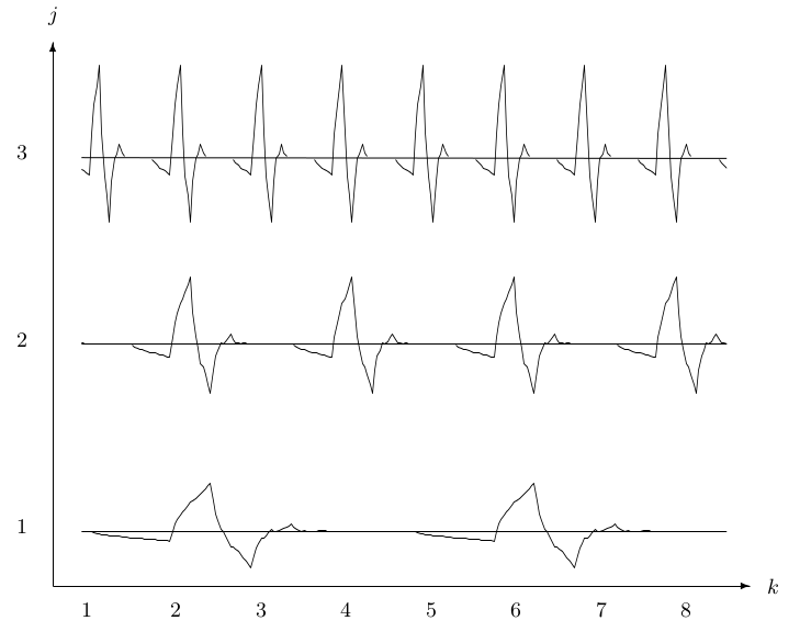
The operations of translation and scaling seem to be basic to many practical signals and signal-generating processes, and their use is one of the reasons that wavelets are efficient expansion functions. Figure 2.3 is a pictorial representation of the translation and scaling of a single mother wavelet described in Equation 2.5. As the index k changes, the location of the wavelet moves along the horizontal axis. This allows the expansion to explicitly represent the location of events in time or space. As the index j changes, the shape of the wavelet changes in scale. This allows a representation of detail or resolution. Note that as the scale becomes finer (j larger), the steps in time become smaller. It is both the narrower wavelet and the smaller steps that allow representation of greater detail or higher resolution. For clarity, only every fourth term in the translation (k=1,5,9,13,⋯) is shown, otherwise, the figure is a clutter. What is not illustrated here but is important is that the shape of the basic mother wavelet can also be changed. That is done during the design of the wavelet system and allows one set to well-represent a class of signals.
For the Fourier series and transform and for most signal expansion systems, the expansion functions (bases) are chosen, then the properties of the resulting transform are derived and
analyzed. For the wavelet system, these properties or characteristics are mathematically required, then the resulting basis functions are derived. Because these constraints do not use all the degrees of freedom, other properties can be required to customize the wavelet system for a particular application. Once you decide on a Fourier series, the sinusoidal basis functions are completely set. That is not true for the wavelet. There are an infinity of very different wavelets that all satisfy the above properties. Indeed, the understanding and design of the wavelets is an important topic of this book.
Wavelet analysis is well-suited to transient signals. Fourier analysis is appropriate for periodic signals or for signals whose statistical characteristics do not change with time. It is the localizing property of wavelets that allow a wavelet expansion of a transient event to be modeled with a small number of coefficients. This turns out to be very useful in applications.
The multiresolution formulation needs two closely related basic functions. In addition to the wavelet ψ(t) that has been discussed (but not actually defined yet), we will need another basic function called the scaling functionϕ(t). The reasons for needing this function and the details of the relations will be developed in the next chapter, but here we will simply use it in the wavelet expansion.
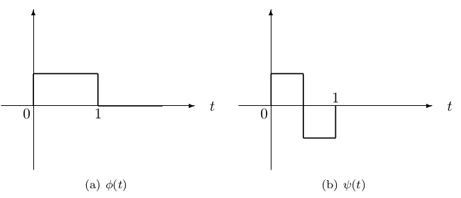
The simplest possible orthogonal wavelet system is generated from the Haar scaling function and wavelet. These are shown in Figure 2.4. Using a combination of these scaling functions and wavelets allows a large class of signals to be represented by

Haar 7 showed this result in 1910, and we now know that wavelets are a generalization of his work. An example of a Haar system and expansion is given at the end of Chapter: A multiresolution formulation of Wavelet Systems.
All Fourier basis functions look alike. A high-frequency sine wave looks like a compressed low-frequency sine wave. A cosine wave is a sine wave translated by 90o or π/2 radians. It takes a
large number of Fourier components to represent a discontinuity or a sharp corner. In contrast, there are many different wavelets and some have sharp corners themselves.
To appreciate the special character of wavelets you should recognize that it was not until the late 1980's that some of the most useful basic wavelets were ever seen. Figure 2.5 illustrates four different scaling functions, each being zero outside of 0<t<6 and each generating an orthogonal wavelet basis for all square integrable functions. This figure is also shown on the cover to this book.
Several more scaling functions and their associated wavelets are illustrated in later chapters, and the Haar wavelet is shown in Figure 2.4 and in detail at the end of Chapter: A multiresolution formulation of Wavelet Systems.

Wavelet expansions and wavelet transforms have proven to be very efficient and effective in analyzing a very wide class of signals and phenomena. Why is this true? What are the properties that give this effectiveness?
The size of the wavelet expansion coefficients aj,k in Equation 2.4 or dj,k in Equation 2.6 drop off rapidly with j and k for a large class of signals. This property is called being an unconditional basis and it is why wavelets are so effective in signal and image compression, denoising, and detection. Donoho 6, 5 showed that wavelets are near optimal for a wide class of signals for compression, denoising, and detection.
The wavelet expansion allows a more accurate local description and separation of signal characteristics. A Fourier coefficient represents a component that lasts for all time and, therefore, temporary events must be described by a phase characteristic that allows cancellation or reinforcement over large time periods. A wavelet expansion coefficient represents a component that is itself local and is easier to interpret. The wavelet expansion may allow a separation of components of a signal that overlap in both time and frequency.
Wavelets are adjustable and adaptable. Because there is not just one wavelet, they can be designed to fit individual applications. They are ideal for adaptive systems that adjust themselves to suit the signal.
The generation of wavelets and the calculation of the discrete wavelet transform is well matched to the digital computer. We will later see that the defining equation for a wavelet uses no calculus. There are no derivatives or integrals, just multiplications and additions—operations that are basic to a digital computer.
While some of these details may not be clear at this point, they should point to the issues that are important to both theory and application and give reasons for the detailed development that follows in this and other books.