In order to talk about the collection of functions or signals that can be represented by a sum of scaling functions and/or wavelets, we need some ideas and terminology from functional analysis. If these concepts are not familiar to you or the information in this section is not sufficient, you may want to skip ahead and read Chapter: The Scaling Function and Scaling Coefficients, Wavelet and Wavelet Coefficients or 11.

A function space is a linear vector space (finite or infinite dimensional) where the vectors are functions, the scalars are real numbers (sometime complex numbers), and scalar multiplication and vector addition are similar to that done in Equation 2.1. The inner product is a scalar a obtained from two vectors, f(t) and g(t), by an integral. It is denoted

(3.1)

with the range of integration depending on the signal class being considered. This inner product defines a norm or “length" of a vector which is denoted and defined by

(3.2)

which is a simple generalization of the geometric operations and definitions in three-dimensional Euclidean space. Two signals (vectors) with non-zero norms are called orthogonal if their inner product is zero. For example, with the Fourier series, we see that sin(t) is orthogonal to sin(2t).

A space that is particularly important in signal processing is call L²(R). This is the space of all functions f(t) with a well defined integral of the square of the modulus of the function. The “L" signifies a Lebesque integral, the “2" denotes the integral of the square of the modulus of the function, and R states that the independent variable of integration t is a number over the whole real line. For a function g(t) to be a member of that space is denoted: g∈L²(R) or simply g∈L².

Although most of the definitions and derivations are in terms of signals that are in L², many of the results hold for larger classes of signals. For example, polynomials are not in L² but can be expanded over any finite domain by most wavelet systems.

In order to develop the wavelet expansion described in Equation 2.5, we will need the idea of an expansion set or a basis set. If we start with the vector space of signals, S, then if any f(t)∈S can be expressed as , the set of functions φ_k(t) are called an expansion set for the space S. If the representation is unique, the set is a basis. Alternatively, one could start with the expansion set or basis set and define the space S as the set of all functions that can be expressed by . This is called the span of the basis set. In several cases, the signal spaces that we will need are actually the closure of the space spanned by the basis set. That means the space contains not only all signals that can be expressed by a linear combination of the basis functions, but also the signals which are the limit of these infinite expansions. The closure of a space is usually denoted by an over-line.

In order to use the idea of multiresolution, we will start by defining the scaling function and then define the wavelet in terms of it. As described for the wavelet in the previous chapter, we define a set of scaling functions in terms of integer translates of the basic scaling function by

(3.3)

The subspace of L²(R) spanned by these functions is defined as

(3.4)

for all integers k from minus infinity to infinity. The over-bar denotes closure. This means that

(3.5)

One can generally increase the size of the subspace spanned by changing the time scale of the scaling functions. A two-dimensional family of functions is generated from the basic scaling function by scaling and translation by

(3.6)

whose span over k is

(3.7)

for all integers k∈Z. This means that if f(t)∈V_j, then it can be expressed as

(3.8)

For j>0, the span can be larger since φ_j,k(t) is narrower and is translated in smaller steps. It, therefore, can represent finer detail. For j<0, φ_j,k(t) is wider and is translated in larger steps. So these wider scaling functions can represent only coarse information, and the space they span is smaller. Another way to think about the effects of a change of scale is in terms of resolution. If one talks about photographic or optical resolution, then this idea of scale is the same as resolving power.

Multiresolution Analysis

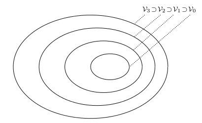
In order to agree with our intuitive ideas of scale or resolution, we formulate the basic requirement of multiresolution analysis (MRA) 6 by requiring a nesting of the spanned spaces as

(3.9) ⋯ ⊂ V _{– 2} ⊂ V _{– 1} ⊂ V₀ ⊂ V₁ ⊂ V₂ ⊂ ⋯ ⊂ L²

or

(3.10)

with

(3.11)

The space that contains high resolution signals will contain those of lower resolution also.

Because of the definition of V_j, the spaces have to satisfy a natural scaling condition

(3.12)

which insures elements in a space are simply scaled versions of the elements in the next space. The relationship of the spanned spaces is illustrated in Figure 3.1.

The nesting of the spans of , denoted by V_j and shown in Equation 3.9 and Equation 3.12 and graphically illustrated in Figure 3.1, is achieved by requiring that φ(t)∈V₁, which means that if φ(t) is in V₀, it is also in V₁, the space spanned by φ(2t). This means φ(t) can be expressed in terms of a weighted sum of shifted φ(2t) as

(3.13)

Figure 3.1. 

Nested Vector Spaces Spanned by the Scaling Functions

where the coefficients h(n) are a sequence of real or perhaps complex numbers called the scaling function coefficients (or the scaling filter or the scaling vector) and the maintains the norm of the scaling function with the scale of two.

This recursive equation is fundamental to the theory of the scaling functions and is, in some ways, analogous to a differential equation with coefficients h(n) and solution φ(t) that may or may not exist or be unique. The equation is referred to by different names to describe different interpretations or points of view. It is called the refinement equation, the multiresolution analysis (MRA) equation, or the dilation equation.

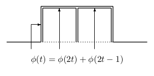
The Haar scaling function is the simple unit-width, unit-height pulse function φ(t) shown in Figure 3.2, and it is obvious that φ(2t) can be used to construct φ(t) by

(3.14)

which means Equation 3.13 is satisfied for coefficients .

The triangle scaling function (also a first order spline) in Figure 3.2 satisfies Equation 3.13 for , and the Daubechies scaling function shown in the first part of

(a)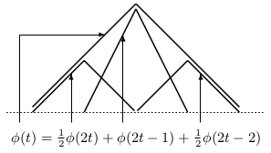

(b)

Figure 3.2. 

Haar and Triangle Scaling Functions

Figure: Daubechies Scaling Functions satisfies Equation 3.13 for h={0.483,0.8365,0.2241,–0.1294} as do all scaling functions for their corresponding scaling coefficients. Indeed, the design of wavelet systems is the choosing of the coefficients h(n) and that is developed later.

The important features of a signal can better be described or parameterized, not by using φ_j,k(t) and increasing j to increase the size of the subspace spanned by the scaling functions, but by defining a slightly different set of functions ψ_j,k(t) that span the differences between the spaces spanned by the various scales of the scaling function. These functions are the wavelets discussed in the introduction of this book.

There are several advantages to requiring that the scaling functions and wavelets be orthogonal. Orthogonal basis functions allow simple calculation of expansion coefficients and have a Parseval's theorem that allows a partitioning of the signal energy in the wavelet transform domain. The orthogonal complement of V_j in V_j+1 is defined as W_j. This means that all members of V_j are orthogonal to all members of W_j. We require

(3.15)

for all appropriate j,k,ℓ∈Z.

The relationship of the various subspaces can be seen from the following expressions. From Equation 3.9 we see that we may start at any V_j, say at j=0, and write

We now define the wavelet spanned subspace W₀ such that

(3.17)

which extends to

(3.18)

In general this gives

when V₀ is the initial space spanned by the scaling function ϕ(t–k). Figure 3.3 pictorially shows the nesting of the scaling function spaces V_j for different scales j and how the wavelet spaces are the disjoint differences (except for the zero element) or, the orthogonal complements.

The scale of the initial space is arbitrary and could be chosen at a higher resolution of, say, j=10 to give

or at a lower resolution such as j=–5 to give