The Fourier Transform can be used to represent any well behaved function f ( x ) .

where A ( k ) = ∫^∞ _{− ∞} f ( x ) cos ( kx ) ⅆ x B ( k ) = ∫^∞ _{− ∞} f ( x ) sin ( kx ) ⅆ x I can now substitute for A and B in the original expression and write:

and then use cos ( x^′ − x ) = c o s k x cos k x^′ + sin kx sin k x^′

Since the inner integral is an even function we can write Now consider the fact that because sin is an odd function, ie. ∫^∞ _{− ∞} sin ( k [ x^′ − x ] ) ⅆ k = 0 So we could have written or or where g ( k ) = ∫^∞ _{− ∞} f ( x ) e^ikx ⅆ x is the Fourier transform of f ( x ) .

Symbolically we write g ( k ) = Ϝ { f ( x ) } f ( x ) = Ϝ ^{− 1} { g ( k ) } = Ϝ ^{− 1} { Ϝ { f ( x ) } }

Now these concepts are easily extended to two dimensions:

where g ( k_x , k_y ) = ∫^∞ _{− ∞} ∫^∞ _{− ∞} f ( x , y ) e^{i ( x k_x + y k_y )} ⅆ x ⅆ y .

This tells us is that any nonperiodic function of two variables f ( x , y ) can be synthesized from a distribution of plane waves each with amplitude g ( k_x , k_y ) .

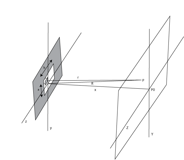
Lets consider Fraunhofer diffraction through an aperture again. For example consider a rectangular aperture as show in the figure. If is the source strength per unit area (assumed to be constant over the entire area in this example) and dS = ⅆ x ⅆ z is an infinitesmal area at a point in the aperture then we have:

Figure 11.1. 

We can define a source strength per unit area

Notice that I flipped the sign in the exponential from what I used in the earlier lectures on diffraction. This does not change the physics content of what we are doing in any way, however it allows our notation to follow standard convention.

If we define k_y = k Y / R and k_z = Z / R and we see that

That is, it is equal to the Fourier transform. In fact one can define an "Aperture Function" A ( y , z ) . Such that

For a rectangular aperture inside the aperture and zero outside it. The aperture function can be much more complex (literally) allowing for changes in source strength and phase through the aperture. The resulting E field is the Fourier transform of the aperture function.

The above allows us to relate the Fourier transform of an Aperture and the resulting E field from diffraction through that aperture. To extend this to an array of apertures, requires that one introduce a new concept, the Dirac delta function.

The fundamental definition of the Dirac delta function is

As a special case if f ( x ) = 1

∫^∞ _{− ∞} δ ( x ) ⅆ x = 1

This function has some important properties:

f ( x^′ ) = ∫^∞ _{− ∞} f ( x ) δ ( x − x^′ ) ⅆ x which follows direction from the definition ie. define a new coordinate a = x − x^′ , then x = a + x^′ and da = ⅆ x . Then

We also note that δ ( x ) = δ ( − x ) .

It gets even more interesting. Recall which we rearrange suggestively we also have f ( x ) = ∫^∞ _{− ∞} f ( x^′ ) δ ( x^′ − x ) ⅆ x^′ so we must have or

That is the Dirac delta function is the inverse Fourier transform of 1. This is a very useful property that allows us to do problems like Young's double slit. Consider the aperture function: A = E₀ ( δ ( y − a / 2 ) + δ ( y + a / 2 ) ) where we have represented the slits by Dirac delta functions. Then we obtain which is exactly what we obtained before. Well that was a lot easier than what we did earlier in the course!