Diffraction is an important characteristic of waves. It can be said to one of the defining characteristics of a wave. It occurs when part of a wavefront is obstructed. The parts of the wavefronts that propagate past the the obstacle interfere and create a diffraction pattern. Diffraction and interference are essentially the same physical process, resulting from the vector addition of fields from different sources. By convention interference refers to only a few sources and diffraction refers to many sources or a continuous source.

Figure 10.1. 

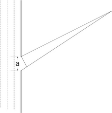
When a plane wave hits an aperture, Huygens principle says that each point in the aperture acts as a source of spherical wavelets. The maximum path length difference of all these sources is between the top and the bottom. Δ r_max = a sinθ The waves start out in phase. If a < < λ then the slit acts as a point source and you get a spherical wave coming out. If a > > λ then the aperture simply casts a bright spot the size of the aperture shadow. But if λ ≈ a then an interference pattern is set up.When the resulting pattern is viewed close to the aperture, the pattern can be very complex, and this is call Fresnel diffraction. As the the pattern is viewed from further and further away, it eventually stops changing shape and only grows in size. This is Fraunhoffer diffraction.

Single Slit Diffraction

Figure 10.2. 

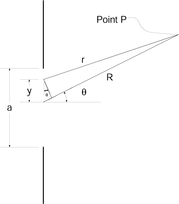
Consider the contribution to the field at a P due to a small element of the slit ⅆ y at y . It is a distance r from P. R is the distance from the center of the slit to P.

lets define ε_L which is the source strength per unit length, which is a constant.

then

Now from the drawing Now assume that y < < R (which gives us the Franhaufer condition) and now expand the square root

and neglect higher terms so that r = R − y sinθ thus where now we have used R in the denominator since it is much bigger than y

now integrate assuming that θ is a constant over the slit

now we define and see that we can rewrite our expression as or equivalently

The intensity will go like the square of this so

I = I₀s i n c²β

Figure 10.3. 

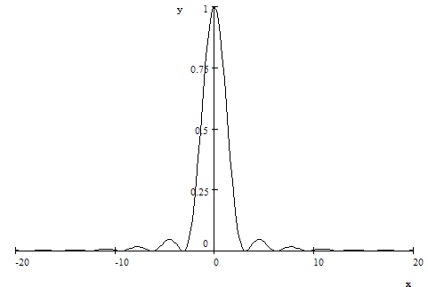
Plot of

The Intensity has a maximum at β = 0 or θ = 0 . there are minima when sinβ = 0 or in the case of small θ we see that is the distance between adjacent minima.

As a becomes large, we see that the minima will merge together. This is consistent with what we said at the beginning, that if a > > λ then you just get shadowing but not diffraction.

Finding the secondary maxima is more difficult. (Take the derivative of I and then look for zeros.) This can not be done analytically.

Note that wee have been considering only one dimension. If the length of the slit is L then we have only considered the case that L > > λ and so diffraction occurs only in the other dimension.

Now we consider the case of two slit diffraction.

Figure 10.4. 

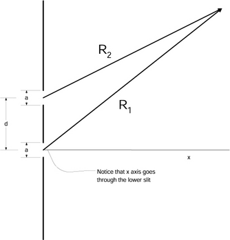
Notice that the x axis has been drawn through the lower slit. Then the field at the distant point is just the sum of the field from the two slits. Thus we can use our solution to single slit diffraction for each slit and add them together

Now we we will define R = R₁ and use R₂ = R − d sinθ Now we can ignore the d sinθ in the denominator, as it will not have a significant effect on that. However in the exponent, we can not ignore it, since it could significantly affect the phase of the harmonic function. Lets define α = ( k d sinθ ) / 2 so now we can write: and start rearranging: This is very similar to the case of single slit diffraction except that you now get a factor 2 cosα included and a phase shift in the harmonic function.

So we can see immediately the intensity is I = 4 I₀ cos²α s i n c²β recall α = ( k d sinθ ) / 2 and β = ( k a sinθ ) / 2 If d goes to 0 then expression just becomes the expression for single slit diffraction. If a goes to 0 then the expression just becomes that for Youngs double slit. The double slit diffraction is just the product of these two results. (Hey cool!)

Consider the case of N slit diffraction, We have . . . So we can just follow the steps of the two slit case and extend them and get (using R_N = R − ( N − 1 ) d sinθ ) This is the same geometric series we dealt with before so

Notice that this just ends up being multisource interference multiplied by single slit diffraction.

Squaring it we see that:

Figure 10.5. 

Interference with diffraction for 6 slits with d = 4 a

Figure 10.6. 

Interference with diffraction for 6 slits with d = 4 a

Figure 10.7. 

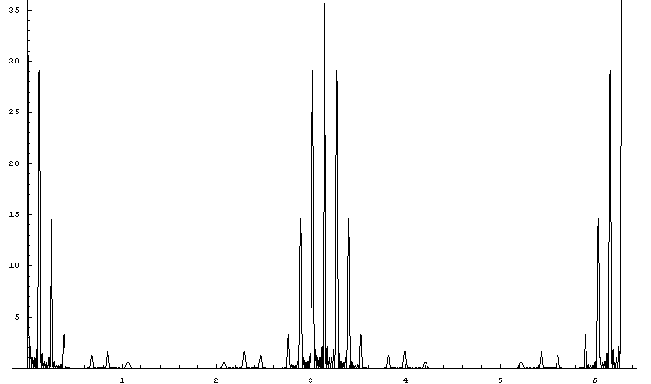
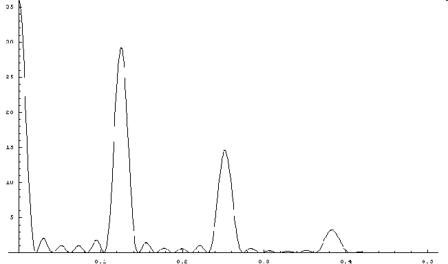
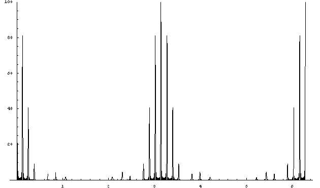
Interference with diffraction for10 slits with d = 4 a

Figure 10.8. 

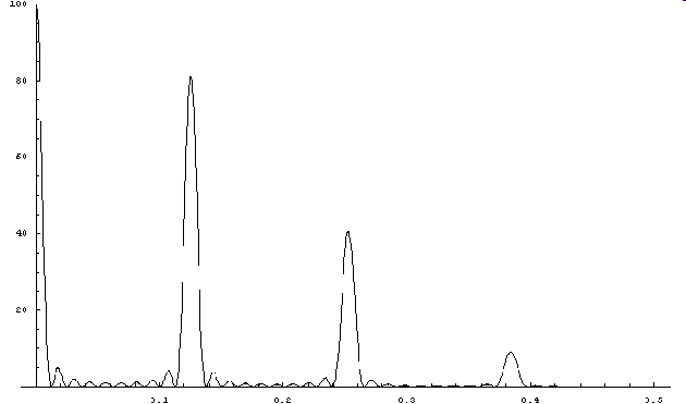
Interference with diffraction for10 slits with d = 4 a

Principal maxima occur when or since α = k d ( sinθ ) / 2 k d sinθ = 2 n π    n = 0 , 1 , 2 , 3 or or

and just like in multisource interference minima occur at A diffraction grating is a repetitive array of diffracting elements such as slits or reflectors. Typically with N very large (100's). Notice how all but the first maximum depend on λ . So you can use a grating for spectroscopy.

We consider diffraction from apertures other than a slit. For example consider a rectangular aperture as shown below. If is the source strength per unit area (assumed to be constant over the entire area in this example) and dS = ⅆ y ⅆ z is an infinitesmal area at a point in the aperture then we have:

Figure 10.9. 

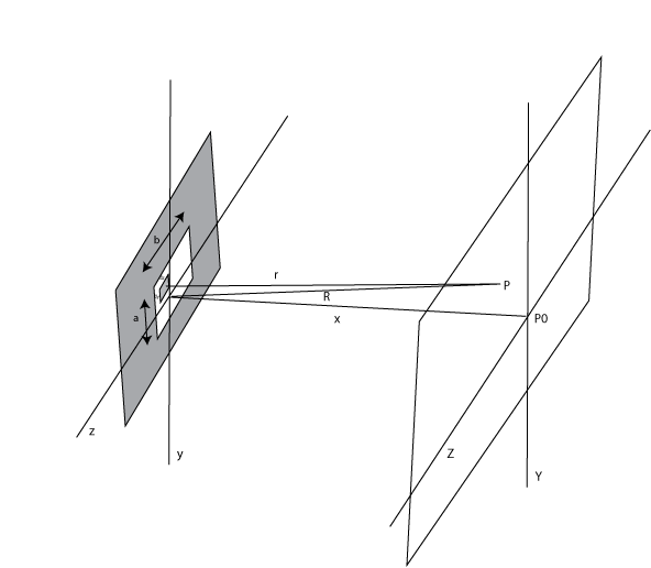
We see from the figure that and that R² = x² + Y² + Z² . Thus we use x² = R² − Y² − Z² to write or We are only considering Fraunhofer diffraction so R , Z , Y are much larger than y and z and we can rewrite and then finally expanding using the binomial theorem and taking only the most significant terms