
Consider the forces on a short fragment of string
Fy
=
T
sin
(
θ
+
Δ
θ
)
−
T
sinθ
Fx
=
T
cos
(
θ
+
Δ
θ
)
−
T
cosθ
Assume that the displacement in y is small and
T
is a constant along the stringthus
θ
and
θ
+
Δ
θ
are smallthen
Fx
≈
0
we can see this by expanding the trig functions
 or
Fx
≈
T
θ
Δ
θ
which is very small.On the other hand
Fy
≈
T
[
θ
+
Δ
θ
−
θ
+
…
]
or
Fy
≈
T
Δ
θ
which is not nearly as small. So we will consider the
y
component of motion, but approximate there is no x component
or
Fx
≈
T
θ
Δ
θ
which is very small.On the other hand
Fy
≈
T
[
θ
+
Δ
θ
−
θ
+
…
]
or
Fy
≈
T
Δ
θ
which is not nearly as small. So we will consider the
y
component of motion, but approximate there is no x component
 Also we can write:
Fy
=
m
ay
m
=
μ
Δ
x
where
μ
is the mass density
Also we can write:
Fy
=
m
ay
m
=
μ
Δ
x
where
μ
is the mass density
 now have

 Note dimensions, get a velocity

 The second space derivative of a function is equal to the second
time derivative of a function multiplied by a constant.
The second space derivative of a function is equal to the second
time derivative of a function multiplied by a constant.
Before considering traveling waves, we are going to look at a special case solution to the wave equation. This is the case of stationary vibrations of a string.
For example here, lets consider the case where both ends of the string are
fixed at
y
=
0
.
Now we vibrate the string. Every point along the string acts like a little
driven oscillator. So lets assume that every point on string has a time
dependence of the form
cos
ωt
and that the amplitude is a function of distance Assume
y
(
x
,
t
)
=
f
(
x
)
cos
ωt
then

 Substitute into wave equation

 Then every
f
(
x
)
that satisfies:
Then every
f
(
x
)
that satisfies:
 is a solution of the wave equation
A solution is (requiring
f
(
0
)
=
0
since ends fixed)
 Another boundary condition is
f
(
L
)
=
0
so get
Another boundary condition is
f
(
L
)
=
0
so get
 Thus
Thus


Be careful with the equations above: v is the letter vee and is for velocity. now we introduce the frequency ν which is the Greek letter nu.
recall
ν
=
ω
/
2
π
so
 This is a very important feature of wave phenomena. Things can be quantized.
This is why a musical instrument will play specific notes. Note, that we
must have an integral number of half sine waves
This is a very important feature of wave phenomena. Things can be quantized.
This is why a musical instrument will play specific notes. Note, that we
must have an integral number of half sine waves
 end up with
 leading to
 where
where
 ω1
is the fundamental frequency
ω1
is the fundamental frequency
In deriving the motion of a string under tension we came up with an equation:
 which is known as the wave equation. We will show that this leads to waves
below, but first, let us note the fact that solutions of this equation can be
added to give additional solutions.
which is known as the wave equation. We will show that this leads to waves
below, but first, let us note the fact that solutions of this equation can be
added to give additional solutions.
Say you have two waves governed by two equations Since they are traveling in
the same medium,
v
is the
same
 add
these
add
these
 Thus
f1
+
f2
is a solution to the wave equation
Thus
f1
+
f2
is a solution to the wave equation
Lets say we have two functions,
f1
(
x
−
v
t
)
and
f2
(
x
+
v
t
)
.
Each of these functions individually satisfy the wave equation. note that
y
=
f1
(
x
−
v
t
)
+
f2
(
x
+
v
t
)
will
also satisfy the wave equation. In fact any number of functions of the form
f
(
x
−
v
t
)
or
f
(
x
+
v
t
)
can be added together and will satisfy the wave equation. This is a very
profound property of waves. For example it will allow us to describe a very
complex wave form, as the summation of simpler wave forms. The fact that
waves add is a consequence of the fact that the wave equation
 is
linear, that is
f
and its derivatives only appear to first order. Thus any linear combination of
solutions of the equation is itself a solution to the equation.
is
linear, that is
f
and its derivatives only appear to first order. Thus any linear combination of
solutions of the equation is itself a solution to the equation.
Any well behaved (ie. no discontinuities, differentiable) function of the form
y
=
f
(
x
−
v
t
)
is
a solution to the wave equation. Lets define
and
Then
using the chain rule
and
Also
 We
see that this satisfies the wave equation.
We
see that this satisfies the wave equation.
Lets take the example of a Gaussian pulse. f ( x − v t ) = A e − ( x − v t ) 2 / 2 σ2
Then

and
or
That is it satisfies the wave equation.
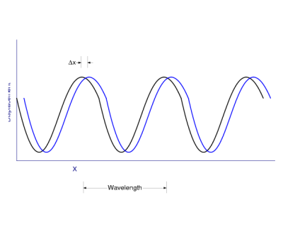
To find the velocity of a wave, consider the wave:
y
(
x
,
t
)
=
f
(
x
−
v
t
)
Then can see that if you increase time and x by
Δ
t
and
Δ
x
for a point on the traveling wave of constant amplitude
f
(
x
−
v
t
)
=
f
(
(
x
+
Δ
x
)
−
v
(
t
+
Δ
t
)
)
.
Which is true if
Δ
x
−
v
Δ
t
=
0
or
Thus
f
(
x
−
v
t
)
describes a wave that is moving in the positive
x
direction. Likewise
f
(
x
+
v
t
)
describes a wave moving in the negative x direction.
Lots of students get this backwards so watch out!
Another way to picture this is to consider a one dimensional wave pulse of arbitrary shape, described by y′ = f ( x′ ) , fixed to a coordinate system O′ ( x′ , y′ )
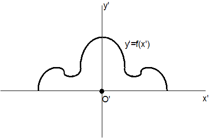
Now let the O′ system, together with the pulse, move to the right along the x-axis at uniform speed v relative to a fixed coordinate system O ( x , y ) .
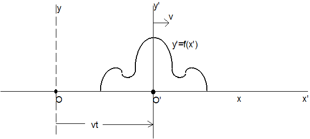
As
it moves, the pulse is assumed to maintain its shape. Any point P on the pulse
can be described by either of two coordinates
x
or
x′,
where
x′
=
x
−
v