It is presumed that the deviations between observed flow pattern and predicted flow behaviour are caused by the turbulence model used. Some authors already compared different
models that simplify turbulent effects by correlation factors and additional equations like the k-ε RNG model. They stated that the k-ε RNG model is a reasonable compromise between
computational demand and validity of the results (Wardle et al., 2006). Other authors relied on the more extensive Reynolds Stress Model (RSM) or the large-eddy simulation (LES) (Mainza
et al., 2006; Wang & Yu, 2006). Nowakowski et al. reviewed the milestones in the application of computational fluid dynamics in hydrocyclones (Nowakowski et al., 2004). The most common
models used are the k-ε and recently the RSM and LES model. For the evaluation of the
differences in the prediction of the flow behaviour in centrifuges between several turbulence models, the flow pattern was calculated for various rotational speeds and throughputs, using the k-e RNG, k-w, Reynolds Stress Model and large-eddy simulation. A representative
comparison of the obtained results by using the different models is shown in Figure 10. The
plots illustrate the differences in the calculated tangential and axial velocity halfway between inlet and outlet at the angular position of the inlet.
Fig. 10. Tangential (left) and axial velocity profiles (right), throughput 1 l/min, k-e RNG, k-w, RSM and LES turbulence model
114
Applied Computational Fluid Dynamics
The comparison reveals no significant deviation of the predicted flow pattern. The differences in the tangential velocity are barely detectable. All calculations are in good agreement with the rigid body rotation and thus with the experimentally determined profiles (Spelter, et al. 2011).
Using the LES model, the obtained axial flow profile differs from the other models by
predicting an earlier shift of the main axial flow towards the radius of the outlet at 36 mm.
Because of the high computational demand and instability of the RSM, the simulation with this turbulence model was started with a solution obtained with the k-e RNG model. Nevertheless
the differences are small and all calculated axial flow pattern are in disagreement with the measured flow profile. The mixing and expanding of the inlet jet is significantly understated.
By not questioning and validating the simulations, the user of the CFD software is led to false conclusions which may result in low performance of the centrifuge due to disadvantageous
design. The classical evaluation of the simulation does not indicate a computational error. The mass balance between the inlet and the outlet is fulfilled as stated in Table 1, the residuals are sufficiently small (10-3 to 10-5) and the flow patterns do not change with increasing flow time.
Furthermore the predictions are reproducible with different turbulence models. All these facts suggest an accurate calculation. Only the comparison of the main velocities with
experimentally determined data shows that the prediction misrepresents the true case in
respect to the axial flow profile.
Model
k-e RNG
k-w
RSM LES
% dV
0.0395 0.0015 0.0022 0.0172
Table 1. Deviation of mass balance dV for different turbulence models in % at 3000 rpm and
1 l/min
4.3 Comparison of two and three dimensional modelling
The analysis of the acceleration geometry is only possible in three dimensional modelling,
because, as mentioned in the introduction, the inlet geometry cannot be correctly
reproduced in the two dimensional case. The results presented in chapter 4.1 and 4.2 show a
short-circuit flow between inlet and outlet. The comparison between the results obtained
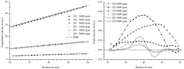
when calculating three and two dimensional are shown in Figure 11. The predicted
tangential velocity profiles are in good agreement with the rigid body rotation for both cases Fig. 11. Tangential and axial velocity profiles, throughput 1 l/min, k-e RNG, k-w, RSM and
LES turbulence model
Computational Fluid Dynamics (CFD) and
Discrete Element Method (DEM) Applied to Centrifuges
115
at various rotational speeds. The water is fed through an annulus in the two dimensional
model and the tangential acceleration takes place via the friction at the wall at both sides of the annulus. According to the prediction, this feeding geometry is sufficient for an
acceleration of the incoming liquid up to 9000 rpm. The differences between the cases are
distinguishable in the axial flow profiles which are shown in the diagram on the right side of Figure 11. The profiles presented are the values halfway between inlet and outlet. Due to the symmetry condition, the flow is homogeneously distributed along the whole circumference
for a specific radius. Therefore the maximum axial velocity is lower than in the three
dimensional case due to the conservation of mass. There are recirculating currents next to
the inlet in the two dimensional cases which increase in magnitude with rotational speed. In the three dimensional case, recirculating flows are located next to the inlet as well, but
displaced few degrees in the angle of rotation.
Nevertheless the predicted axial velocity profiles in the two dimensional cases are
comparable to the ones obtained in the three dimensional ones in respect to the radial
distribution of the flow. The inlet jet remains until the water leaves the centrifuge via the circular weir, so that no plug-shaped profile - resulting in a high active volume -, as
observed in the experiments, is formed.
4.4 Calculation of the flow pattern (k-e RNG model, VOF method, transient solution) -
overflow setup
The overflow setup was simulated by using the previously described Volume of Fluid
method. The centrifuge is filled with water at the beginning of the simulation. As an initial condition, the water is already spinning with the rigid body rotation. This assumption is
justifiable because in the experiments, the centrifuge was slowly filled with water and ran
for at least 30 minutes in steady state prior to the measurements. The initial condition
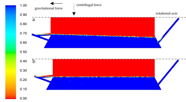
reduces the necessary time until the steady state is reached significantly. Figure 12 shows
Fig. 12. Profiles of water-air interface for a throughput of 1 l/min: a) 1000 rpm; b) 9000 rpm the distribution of the two phases for 1000 (a) und 9000 rpm (b) for a throughput of 1 l/min.
Due to the gravitational and centrifugal force, a conical shape of the water surface is
developed at 1000 rpm. The centrifugal number outbalances the gravitational force with


116
Applied Computational Fluid Dynamics
increasing rotational speed, thus the water phase approaches the shape of a cylinder, as
shown in Figure 12 b).
The tangential velocity profiles for 1000 and 9000 rpm are shown in Figure 13. The diagram
on the right side shows the tangential velocity values averaged over the length of the
centrifuge for the water phase only. The computed values are compared to the rigid body
rotation. The contours of the tangential velocity at 9000 rpm are shown on the left side of
Figure 13. The calculated velocities are in good agreement with the analytical values and
with the measurements. At 9000 rpm, the tangential velocity of the water exhibits a small lag when compared to the rigid body rotation. The magnitude of the deviation is within the
accuracy of the measurements, so that no statement whether this difference is the true case
or not, is possible.
Fig. 13. Tangential velocity profiles, water phase, throughput of 1 l/min; left: contours at 9000 rpm; right: for different rotational speeds and different axial positions
Figure 14 shows the axial velocity profiles for 9000 rpm at a constant throughput of 1 l/min.
The axial flow pattern is similar to the one predicted in the single-phase model. The inlet jet Fig. 14. Axial velocity profiles at 9000 rpm and 1 l/min throughput; left: contours; right:
different distances from the inlet
Computational Fluid Dynamics (CFD) and
Discrete Element Method (DEM) Applied to Centrifuges
117
does not widen so that a short-circuit flow towards the outlet is formed, as shown in the
contour plot on the left side of Figure 14. There is no significant expansion of the flow
profile neither in angular nor in radial direction. The peak of the axial velocity shifts from a radius of 42 mm close to the inlet towards a radius of 36 mm. This behaviour was also
predicted in the single-phase model. Nevertheless the simulation misrepresents the true
case, in which a significant widening of the inlet jet was observed.
4.5 Influence of the inlet geometry on the flow pattern
In order to investigate how the acceleration of the feed affects the flow pattern, a centrifuge with a simpler geometry and a low performance feed accelerator was simulated. The main
differences when compared to the tubular bowl centrifuge are the lower length-to-diameter
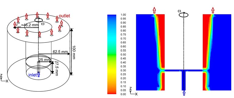
ratio of 0.8 and the feed accelerator. The feed enters a rotating disc and leaves it radially with a certain angular velocity. The water exits the centrifuge through eight boreholes
distributed along the circumference at the top of the bowl. Figure 15 shows a scheme of the
centrifuge geometry on the left and the results of the volume fraction of air on the right.
Water is fed axially through the inlet to the accelerator; there, the water changes its direction and gains in tangential velocity. The transfer of rotational movement occurs just at the plate surfaces, defined as no-slip boundaries, via momentum diffusion. Then, the water exits the
accelerator as streams that travel through the air core and enter the rotating liquid pool. The radius of the interface changes 35 % along the height of the centrifuge from the inlet to the upper part of the centrifuge because of the low rotational speed (454 g).
Fig. 15. Left: geometry of the centrifuge; right: contours of volume fraction of air at 2550 rpm and 5.8 l/min
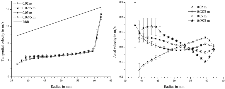
The main flow occurs in the direction of the rotation of the bowl. Both, the liquid pool and the air core rotate. The tangential velocity of the water jet from the inlet accelerator (height 0.0275 m) is lower than the tangential velocity of the bowl. This causes a drag of the whole rotating liquid pool regarding the angular velocity of the bowl. The values of the tangential velocity of the liquid averaged over the circumference are plotted for different heights in
Figure 16. The averaged velocity of the liquid in this geometry is approximately 50 % below
the rigid body rotation. The values at the wall have to match the rigid body rotation of the bowl to fulfil the no-slip boundary condition. The steep decrease of the tangential velocity
118
Applied Computational Fluid Dynamics
near the wall was found to be smoother for a 6 times finer grid. However, the computational
effort for the multiphase simulation including the particles with the finer grid was
unaffordable. The deviation with respect to the rigid body rotation decreases for lower flow rates because a smaller amount of liquid has to be accelerated. The simulation of this
geometry shows how important is to accelerate the feed properly to the angular velocity of
the liquid pool before entering it in order to reach the angular velocity of the bowl in the rotating liquid and thus the highest centrifugal acceleration possible.
In contrast to the other centrifuge, a layer with high axial velocity at the gas-liquid interface, as expected by the boundary layer model, has been observed in the simulations as depicted
in the diagram on the right in Figure 16. Near the impact height of the inlet water jet two
whirls with opposed directions are formed. This can be seen at the negative axial velocity
values at the interface for the height 0.02 m, just below the inlet, and the positive axial
velocities at he interface for the height 0.0275 m, just above the inlet. Upsides the height of the inlet, a homogeneous axial boundary layer is formed at the interface with a
recirculation layer at the bowl wall. This layer exhibits a similar averaged thickness δ as
the one proposed by the theoretical model of Gosele (Gösele, 1968) but much thicker as
the one calculated following the theory of Reuter (Reuter, 1967) as seen in Table 2. Indeed, it occupies the whole liquid pool until a recirculation layer is formed close to the bowl
wall. This is due to the lower tangential velocities which cause a small pressure gradient
in the radial direction reducing the stratification of the flow and allowing the fluid to
move in the axial direction. The velocity values oscillate with the angle, especially near
the inlet at 0.02 m and 0.0275 m and the outlet at 0.0975 m, respectively. Thus the standard deviation is higher at these positions.
Fig. 16. Left: tangential velocity versus radial position; right: axial velocity versus radial position at 2550 rpm and 5.8 l/min
δsimulated (mm)
δReuter (mm)
δGösele (mm)
14.1 1.71
15.8
Table 2. Thickness of the axial boundary layer δ obtained in the simulations and calculated
analytically at 2550 rpm and a throughput of 5.8 l/min
Computational Fluid Dynamics (CFD) and
Discrete Element Method (DEM) Applied to Centrifuges
119
5. Mathematical formulation of the particles
There are several multiphase models available for simulation of a particulate phase. A
summary of the different simulation methods for multiphase flows in CFD can be found in
(van Wachem & Almstedt, 2003). The multiphase models can be divided into two groups;
the Euler-Euler and the Euler-Lagrange methods.
The Euler-Euler method considers all phases as continuous ones. For each phase, a
momentum conservation equation is solved. In the momentum equation of the dispersed
phases, the kinetic theory for granular flows (Lun & Savage, 1987) is used. The intensity of the particle velocity fluctuations determines the stresses, viscosity, and pressure of the solid phase. The interaction between phases is considered by means of momentum exchange
coefficients. This numerical method has the advantage that it is suitable for high volume
concentrations of the disperse phase. The disadvantage is that the properties of each
dispersed particle cannot be simulated and a particle size distribution cannot be considered.
Moreover, the stability of the calculation depends on the choice of model parameters and
often convergence problems appear. For the simulation of sedimentation and thickening
processes there are also some Euler-Euler models based on the Kynch’s kinematics
sedimentation theory (Kynch, 1952), which were reviewed by Bürger in (Bürger &
Wendland, 2001). These models are all based on the measurement of fundamental material
properties of the suspension to be separated as explained by (Buscall, 1990; Buscall et al., 1987; Landman & White, 1994). These multiphase models are based on mass balances for the fluid and the disperse phase. The fluid flow is not calculated but they consider the relative velocity between fluid and particles. On this basis, these models are unsuitable for studying the particle behaviour in solid bowl centrifuges where the liquid flow plays a crucial role in particle settling. These models usually describe the sedimentation and consolidation in
batch processes in simple-geometry centrifuges. An extension of these models is necessary
to describe the sediment build-up in two and three dimensions correctly.
The Euler-Lagrange method solves the continuum conservation equations just for the
characterization of the continuous phase. It describes the dispersed phase as mass points
and determines the particle trajectories by integrating a force balance for each individual
particle. This way, instead of a partial differential equation, only an ordinary differential equation must be solved for the dispersed phase. The weakness of the Euler-Lagrange
method is that it is only valid for diluted suspensions if a one-way or a two-way coupling
method between continuous and disperse phase is applied. With the one-way coupling, the
motion of the discrete phase is calculated based on the velocity field of the continuous phase but the particles have no effect on the pressure and velocity field of the continuous phase. By using a two-way coupling, the equations of continuous and discrete phase are calculated
alternatively. The momentum conservation equation of the continuous phase has a source
term to consider the momentum exchange with the particulate phase. The maximum value for
the volume concentration of the disperse phase is between 5% (Schütz et al., 2007) and 10-12%
(ANSYS, 2009), above this value the interaction between particles should be considered. Thus there is a third method, four-way coupling, which involves the interaction within the disperse phase: impacts between particles, particle-wall interactions, van der Waals forces, electrostatic forces, etc. Thus the restriction for the volume fraction is not valid anymore. However, if the number of particles increases, the computational effort rises significantly. Usually the
characteristics of the problem and the information that should be obtained from the simulation decide which multiphase model and coupling methodology should be used.


120
Applied Computational Fluid Dynamics
The Discrete Element Method (DEM) (Cundall & Strack, 1979) is a Lagrangian method
originally developed for the simulation of bulk solids and then extended to the entire field of particle technology. This method solves the Newton's equations of motion for translation
and rotation of the particles. In these equations, impact forces of particle-particle and
particle-wall interactions are considered. Other forces such as electrostatic or Brownian
forces can also be implemented if necessary. In order to describe the collisions of particles, the soft-sphere approach was chosen. When two particles collide, they actually deform. This
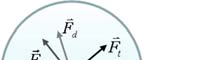
deformation is described by an overlap displacement of the particles. A schematic
representation of the forces on the particles in the soft-sphere model is depicted in Figure 17.
This approach uses a spring-dashpot-slider system to calculate the behaviour of the particles during the contact time. The soft-sphere model allows contacts of a particle with more
neighbouring particles during a time step. The net contact force acting on a particle is added in the case of multiple overlapping. This model for contact forces was first developed by
Cundall (Cundall & Strack, 1979), who proposed a parallel linear spring-dashpot model for the normal direction and a parallel linear spring-dashpot in a series with a slider for the
tangential direction. A comparison of the performance of several soft-sphere models can be
found in (Di Renzo & Di Maio, 2005; Stevens & Hrenya, 2005). There, also the Hertz-Mindlin (Mindlin, 1949) non-linear soft-sphere model used in the present work is analysed. This
model proposes a normal force as a function of the normal overlap δn, the Young’s modulus
of the particle material and the particle radii. The damping force in normal direction
depends on the restitution coefficient, the normal stiffness, and the normal component of the relative velocity between the particles. The tangential force depends on the tangential
overlap δt, on the shear modulus of the particle material, and on the particle radii; while in the damping force in tangential direction the tangential stiffness and the tangential
component of the relative velocity between the particles are considered.
Fig. 17. Contact forces between two particles following the soft-sphere model
While the DEM model was originally used in environments without fluid, increasing efforts
have been made to extend this model to the mixture of fluid and particles. For that, a coupling of the DEM calculations with the fluid flow simulation is necessary to be able to
include the hydrodynamic forces in the particle simulation. An important aspect in the
calculation of particles in a fluid is the energy dissipation into the surrounding fluid. In viscous fluids, there are, in contrast to air, two additional effects that lead to energy losses.
The drag force leads to lower particle velocities and when a particle is about to hit a surface or another particle, a deceleration occurs. This is due to the drainage of the fluid, which is located in the gap between the two particles or the particle and the surface. In his work
Computational Fluid Dynamics (CFD) and
Discrete Element Method (DEM) Applied to Centrifuges
121
(Gondret et al., 2002), Gondret presents the coefficient of restitution as a function of the Stokes number St (Equation 16), which describes the ratio of the dynamic response time of a
particle to flow changes and the characteristic flow time. He determined empirically a
critical Stokes number of about 10. Below this value, a particle does not bounce when it hits a wall and instead remains in contact with it.
1 sv x
St
(16)
9
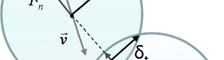
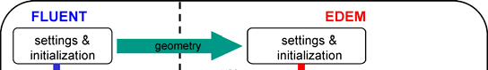
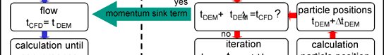
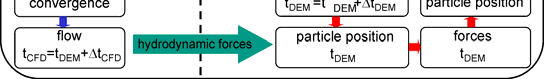
In a centrifugal field, the hydrodynamic forces (drag, lift, torque) play a crucial role and must be included in the calculation of the particle trajectories. Therefore the fluid flow and particles movement have to be computed alternatively. A scheme of the coupling between
the CFD software FLUENT and the DEM software EDEM can be seen in Figure 18. At first,
the flow will be determined with CFD, then for each position in the computational domain,
the velocity, pressure, density and viscosity of the flow are transferred to DEM in order to calculate the hydrodynamic forces and include them in the balance. Afterwards, the fluid
flow will be computed again considering the influence of the particles as an additional sink term in the momentum equations. This sink term include the force transmitted to the
particles by the fluid.
Fig. 18. Coupling between CFD and DEM
Some authors have already simulated such complex multiphase flows in other separation
equipment such as filters and hydrocyclones (Chu et al., 2009; Chu & Yu, 2008; Dong et al., 2003; Ni et al., 2006). Nevertheless due to the high velocity gradients and complex
interactions between the phases, the simulation of multiphase flow and in particular the
sediment behaviour in centrifugal field is still an unsolved challenge. The advantage of this approach is that an accurate description of the flow, the particle paths and the sediment
behaviour can be obtained. However, the amount of simulated particles and its size is
limited due to the computational demand.
5.1 Particles simulation parameters
The calculation in CFD must be run as an unsteady case when coupled with DEM. The DEM
time steps are typically smaller than the CFD time steps in order to correctly capture the
contact behaviour. The choice of time steps in DEM simulation is of great importance in
order to achieve stability in the calculation but does not perform very long calculations,
although still representing the real particle behaviour. Therefore it is necessary to analyse 122
Applied Computational Fluid Dynamics
the forces acting on the particles to determine the different time scales. In the case presented, the Hertzian contact time - the total time of contact in Hertz theory of elastic collision -, the particle sedimentation time - the time required for a particle to settle one diameter -, and the particle relaxation time - the time for a particle to adapt to the surrounding fluid flow - are considered. On the basis of these, the smallest time step must be chosen so that all physical phenomena are represented. In the simulations presented, the Hertzian contact time is the
smallest time scale and, thus a time step tDEM = 10-6 s was chosen in the DEM softwa