328
Applied Computational Fluid Dynamics
Where
p is the volume fraction of solid phase and p,max is maximum packing limit.
The tensor parameters are determined by the granular kinetic theory. The viscous stress
tensor comprises stresses due to the shearing viscosity and the bulk viscosity, resulting from the exchange of quantity of movement due to the movement of the particles and their
collision. A component that results from the friction between the particles can be included to calculate the effects that occur when the solid phase reaches maximum volumetric fraction.
The collisional, kinetic, and frictional effects are added to give the shearing viscosity of the solid phase ( p ):
p
p, col
p, kin
p, fr
(24)
Collisional effect (Eq. 25) and kinetic contribution (Eq. 26) are described by Gidaspow et al.
(1992):
1
2
4
p
p, col
p pdp g 0, pp 1
epp
(25)
5
10
pdp
p
4
p kin
g
e
(26)
96
p 1
epp
1
pp p 1
pp 2
,
0,
g
5
0, pp
The bulk viscosity ( s ) comprises the resistance of the particles of the granular phase to compression and expansion. Equation (27) can be used for this viscosity, according to Lun et al. (1984):
1
2
4
p
(27)
s
p pdp g 0, pp 1
epp
3
In dense low velocity solid phase flows, in which the solid fraction is close to the maximum packing limit, the generation of stresses results mainly from the friction between the
particles. One of the forms to calculate the effect of friction in the stresses is using Eq. (28) (Schaeffer, 1987), where is the internal friction angle and I 2 D is the second invariant of the stress tensor.
p sin
p
p, fr
(28)
2 I 2 D
In granular flows with high volumetric fractions of solids, the effects of collisions between particles become less important. The application of the granular kinetic theory in such cases would, therefore, be less relevant, as the effect of friction between the particles must be taken into account. To overcome this problem, the software Fluent® used a formula of the effect of friction extended for the combined application with the granular flow kinetic theory.
Stresses due to friction between particles are normally written in Newtonian form following
Eq. 29, where friction represents the stress due to frictional effects.
P
I
u u T
friction
friction
friction
p
p
(29)
Use of Fluid Dynamic Simulation to Improve the Design of Spouted Beds
329
The resulting stress of the friction effects is added to the stress derived from the kinetic theory when the volumetric fraction of the solids exceeds a certain critical value. This value is normally considered as 0.5 when the flow is three-dimensional and the value of the
packing limit of the solid phase is 0.63, thus:
p
P
ki
P netic
f
P riction
(30)
p
kinetic
friction
(31)
The pressure due to friction is obtained mainly by semi-empirical form. The viscosity can be obtained by applying the modified Coulomb law, which gives the expression:
P
sen
friction
friction
(32)
2 I 2 D
The friction pressure can be determined with the model described by (Johnson & Jackson, 1987):
j
p
p,min
fr
P iction Fr
(33)
k
p,max
p
where the coefficients are j =2 and k =3 (Ocone et al., 1993). The friction coefficient is assumed to be a function of the volumetric fraction of the solids (Eq. 34) and the viscosity of friction is thus given by Eq. 35.
Fr 0,1 p
(34)
P
sin
friction
friction
(35)
Granular temperature of the solid phase ( ) is proportional to the kinetic energy produced
p
by the random movement of the particles. This effect can be represented by:
3
p p p v
p p p p
p I
p :
v
k
(36)
2
p
p
p
p
t
p
qp
where
p I : represents the generation of the energy by the stress tensor of the p
v
p
p
solid phase; k represents the energy diffusion ( k
p
p
is the diffusion coefficient);
p
represents the energy dissipation produced by collisions and
represents the energy
p
qp
exchange between the solid and the fluid phases.
The diffusion coefficient is given by Gidaspow et al. (1992):
2
150
pdp
p
6
2
s
k
g
e
d
e
g
(37)
p
3841 e
1
p 0, pp 1
pp
2 p p p 1 pp 0,
g
5
pp
pp
0, pp
Dissipation of energy due to the collisions can be described by the expression from Lun
p
et al. (1984):
330
Applied Computational Fluid Dynamics
12
2
1 epp g 0, pp
3
2
2
(38)
p
p p p
d
p
The energy exchange between the solid and the fluid phases due to the kinetic energy of the
random movement of the particles qp is given by Gidaspow et al. (1992):
3 K
qp
qp p
(39)
To solve the equation of granular temperature conservation using the software Fluent®,
three methods are possible, besides the addition of a user function (UDF):
Algebraic: obtained by leaving out the convection and diffusion terms of Eq. 36;
Solution of the partial differential equation: obtained by solving Eq. 36 with all terms,
and
Constant granular temperature: useful in dense phase situations in which the particle
fluctuation is small.
2.2.3 Boundary conditions
For the granular phase p , it is possible to define the shearing stress on the wall as follows:
3
p
g
p
U
(40)
6
p 0
p
s, w
p,max
where: U - velocity of the particle moving parallel to the wall; - specularity coefficient.
s, w
For the granular temperature, the general contour condition is given by (Johnson &
Jackson, 1987):
p
3
q
3
g U
p
s
p 0
p
s,
3
w
1 2 epw g 2
(41)
6
4
p 0 p
p,max
p,max
With the model developed here, it is possible to simulate the fluid dynamic behavior of several gas-solid flow systems, especially dense phase systems, for which the Eulerian approach is
most used. The next section presents some of the most relevant current work in literature on the application of CFD to multiphase flow problems with the Eulerian approach.
3. Numerical simulation of the semi-cylindrical spouted bed
It is impossible to observe the spout channel in a cylindrical bed as the channel is
surrounded by the (particle dense) annular zone. Consequently, the semi-cylindrical
spouted bed arose as an alternative for obtaining experimental measurements for cylindrical
spouted beds. This old technique was first used in a study by Mathur & Gishler (1955). This bed should not be classified as unconventional equipment as its purpose is to obtain
experimental data relating to a full bed with similar geometric characteristics.
As shown in the diagram in Fig. 1, it is possible to obtain a semi-cylindrical bed by placing a transparent wall in a full column bed. The great advantage of constructing a semi-cylindrical spouted bed is that it makes it possible to view the internal behavior of the
particles in the vessel as the spouted channel is in direct contact with the flat wall. From the Use of Fluid Dynamic Simulation to Improve the Design of Spouted Beds
331
supposition that the hydrodynamic behavior of the semi-cylindrical bed is similar to that of a cylindrical bed (for systems with similar geometric characteristics), one can infer
experimental data for cylindrical beds from the data obtained for the half column (velocity
of solids from image analysis, radius of the spout channel, fountain shape). After its first use, even with the caution recommended by its creators, some later studies, notably by
Lefroy & Davidson (1969), suggested that the semi-cylinder did not show significant
differences for the most general designs to which it should be applied.
D
Dc
D
c
Dc c
Pare
Flde plana
at wall
H
H
H
cil
cyl
Hcyl
cil
Dc – column diameter
H
H
Hcon
cone
co
n
Hcone
Di – inlet orifice diameter
Hcyl – cylindrical section height
Hcon – conical section height
Di
Di
Di
Di
Cilíndr
Cylind ico
ric
al
Sem
Semii-cil
-c in
yl d
in ric
dri o
c al
Fig. 1. Diagram of a semi-cylindrical (half-column) spouted bed
It is acknowledged that the insertion of a flat wall into a spouted bed causes significant
modifications to the geometry of the equipment. He et al. (1994a) experimentally evaluated
the hydrodynamic behavior of cylindrical and semi-cylindrical spouted beds with similar
geometry. They observed that inserting the flat wall into the bed changed the velocity
profile of the particles due to the additional system friction caused by the wall. In addition to the above study, He et al. (1994b) studied the behavior of the spouted bed porosity
profile, comparing the results obtained for cylindrical and semi-cylindrical beds. It was
verified that inserting the flat wall did not significantly change the porosity behavior of the bed in comparison with the change caused by the wall on the velocity profile of the solid.
These results, along with others in the literature, raise a question about the semi-cylindrical spouted bed: are the measurements obtained using the half-bed technique truly
representative for inferring the hydrodynamic data for cylindrical beds and, if so, for which variables? The studies by He et al. (1994a, 1994b) are conclusive regarding the velocity of the solid phase and the porosity of the bed, indicating that special care is necessary when
applying this technique. Despite the need for special care, visual information related to the hydrodynamic behavior of the cylindrical bed can only be obtained using the half-column
technique. To analyze these effects, some numerical studies were carried out and the results are discussed in the following chapters.
3.1 Numerical evaluation of the specularity coefficient
Various authors have described the importance of friction between the particulate phase and
the flat wall present in the half-column spouted bed. In view of this effect and the possibility 332
Applied Computational Fluid Dynamics
of evaluating it numerically using CFD numerical simulation, this chapter presents the
results of a numerical study involving the specularity coefficient (a parameter added to the Eulerian model of the particulate phase to represent the friction between this phase and the glass wall in the spouted bed). Experimental results were used to verify the simulation
results in one of the cases. In addition to the results, the characteristics of the computational mesh adopted are presented together with the most relevant aspects of the numerical
solution procedure.
3.1.1 Experimental data
The experimental data presented in this study were obtained for a spouted bed operating
with air spheres at a controlled temperature. Table 1 presents the geometric and operational parameters for the spouted beds, together with the physical characteristics of the phases
present in the equipment.
Semi-cylindrical Conical Spouted Bed
Dc (m)
Column diameter
0.30
Di (m)
Inlet orifice diameter
0.05
Hcon (m)
Conical section height
0.23
Hcyl (m)
Cylindrical section height
0.80
He (m)
Static bed height
0.23
Φ (º)
Conical section angle
60.0
dp (m)
Particle diameter
2.18
ui (m/s)
Velocity inlet
18.0
Tair (ºC)
Air temperature
50.0
ρp (kg/m3)
Solid density
2,512
Table 1. Parameters and geometric characteristics of the equipment used in this study
The experimental evaluation of the hydrodynamics of the spouted beds involved
determining experimental data for a semi-cylindrical spouted bed operating under the
conditions described in Table 1. The velocity of the particles in the annular, spout and
fountain zones were obtained from videos filmed through the glass wall at different axial
and radial positions of the half-column conical spouted bed. To be able to make
measurements using the image analysis software, the software was first calibrated using
standard scales. After being calibrated, the local velocity of the solid was calculated by
analysis of the distance covered by the particle and the time taken to cover the distance.
A static pressure probe was fixed to the upper part of the bed with its point inside. By
varying the position of the probe, the inner pressure of the bed was mapped. Note that the
radial pressure data was obtained in the direction perpendicular to the glass wall in the
semi-cylindrical spouted bed.
The height of the fountain was obtained from the images of the half-column conical
spouted bed. These images were produced using a digital stills camera. Image software
was also used to process the images and obtain the shape of the spout channel and the
height of the fountain.


Use of Fluid Dynamic Simulation to Improve the Design of Spouted Beds
333
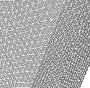
3.2 Computational mesh and numerical procedure
3.2.1 Computational mesh
The simulations were conducted using a three-dimensional mesh containing a symmetry
plane to divide the domain. GAMBIT 2.13 software was used to generate the mesh. The
spacing between nodes adopted was 5.0 mm, increasing gradually towards the outlet zone,
where a spacing of 1.0 cm was adopted. The mesh used tetrahe