sin (5.0º)
=
L y
T L
T L y = T L sin (5.0º) = T sin (5.0º)
T
sin (5.0º)
=
R y
T R
T R y = T R sin (5.0º) = T sin (5.0º).
Now, we can substitute the values for T L y and T R y , into the net force equation in the vertical direction:
F
(4.50)
net y
= T L y + T R y − w = 0
F net y
= T sin (5.0º) + T sin (5.0º) − w = 0
2 T sin (5.0º) − w = 0
2 T sin (5.0º)
= w
and
(4.51)
T =
w
2 sin (5.0º) =
mg
2 sin (5.0º),
so that
(4.52)
T = (70.0 kg)(9.80 m/s2)
2(0.0872)
,
and the tension is
T
(4.53)
= 3900 N.
Discussion
Note that the vertical tension in the wire acts as a normal force that supports the weight of the tightrope walker. The tension is almost six times
the 686-N weight of the tightrope walker. Since the wire is nearly horizontal, the vertical component of its tension is only a small fraction of the
tension in the wire. The large horizontal components are in opposite directions and cancel, and so most of the tension in the wire is not used to
support the weight of the tightrope walker.
If we wish to create a very large tension, all we have to do is exert a force perpendicular to a flexible connector, as illustrated in Figure 4.19. As we saw in the last example, the weight of the tightrope walker acted as a force perpendicular to the rope. We saw that the tension in the roped related to
the weight of the tightrope walker in the following way:
(4.54)
T =
w
2 sin ( θ).
We can extend this expression to describe the tension T created when a perpendicular force ( F⊥ ) is exerted at the middle of a flexible connector:
(4.55)
T = F⊥
2 sin ( θ).
Note that θ is the angle between the horizontal and the bent connector. In this case, T becomes very large as θ approaches zero. Even the
relatively small weight of any flexible connector will cause it to sag, since an infinite tension would result if it were horizontal (i.e., θ = 0 and
sin θ = 0 ). (See Figure 4.19.)

CHAPTER 4 | DYNAMICS: FORCE AND NEWTON'S LAWS OF MOTION 141
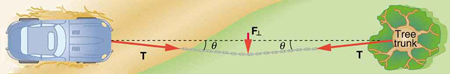
Figure 4.19 We can create a very large tension in the chain by pushing on it perpendicular to its length, as shown. Suppose we wish to pull a car out of the mud when no tow
truck is available. Each time the car moves forward, the chain is tightened to keep it as nearly straight as possible. The tension in the chain is given by T =
F⊥
2 sin ( θ) ;
since θ is small, T is very large. This situation is analogous to the tightrope walker shown in Figure 4.17, except that the tensions shown here are those transmitted to the
car and the tree rather than those acting at the point where F⊥ is applied.
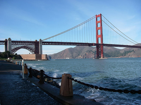
Figure 4.20 Unless an infinite tension is exerted, any flexible connector—such as the chain at the bottom of the picture—will sag under its own weight, giving a characteristic
curve when the weight is evenly distributed along the length. Suspension bridges—such as the Golden Gate Bridge shown in this image—are essentially very heavy flexible
connectors. The weight of the bridge is evenly distributed along the length of flexible connectors, usually cables, which take on the characteristic shape. (credit: Leaflet,
Wikimedia Commons)
Extended Topic: Real Forces and Inertial Frames
There is another distinction among forces in addition to the types already mentioned. Some forces are real, whereas others are not. Real forces are
those that have some physical origin, such as the gravitational pull. Contrastingly, fictitious forces are those that arise simply because an observer is
in an accelerating frame of reference, such as one that rotates (like a merry-go-round) or undergoes linear acceleration (like a car slowing down). For
example, if a satellite is heading due north above Earth’s northern hemisphere, then to an observer on Earth it will appear to experience a force to the
west that has no physical origin. Of course, what is happening here is that Earth is rotating toward the east and moves east under the satellite. In
Earth’s frame this looks like a westward force on the satellite, or it can be interpreted as a violation of Newton’s first law (the law of inertia). An
inertial frame of reference is one in which all forces are real and, equivalently, one in which Newton’s laws have the simple forms given in this
chapter.
Earth’s rotation is slow enough that Earth is nearly an inertial frame. You ordinarily must perform precise experiments to observe fictitious forces and
the slight departures from Newton’s laws, such as the effect just described. On the large scale, such as for the rotation of weather systems and ocean
currents, the effects can be easily observed.
The crucial factor in determining whether a frame of reference is inertial is whether it accelerates or rotates relative to a known inertial frame. Unless
stated otherwise, all phenomena discussed in this text are considered in inertial frames.
All the forces discussed in this section are real forces, but there are a number of other real forces, such as lift and thrust, that are not discussed in this
section. They are more specialized, and it is not necessary to discuss every type of force. It is natural, however, to ask where the basic simplicity we
seek to find in physics is in the long list of forces. Are some more basic than others? Are some different manifestations of the same underlying force?
The answer to both questions is yes, as will be seen in the next (extended) section and in the treatment of modern physics later in the text.
PhET Explorations: Forces in 1 Dimension
Explore the forces at work when you try to push a filing cabinet. Create an applied force and see the resulting friction force and total force acting
on the cabinet. Charts show the forces, position, velocity, and acceleration vs. time. View a free-body diagram of all the forces (including
gravitational and normal forces).
Figure 4.21 Forces in 1 Dimension (http://cnx.org/content/m42075/1.4/forces-1d_en.jar)
142 CHAPTER 4 | DYNAMICS: FORCE AND NEWTON'S LAWS OF MOTION
4.6 Problem-Solving Strategies
Success in problem solving is obviously necessary to understand and apply physical principles, not to mention the more immediate need of passing
exams. The basics of problem solving, presented earlier in this text, are followed here, but specific strategies useful in applying Newton’s laws of
motion are emphasized. These techniques also reinforce concepts that are useful in many other areas of physics. Many problem-solving strategies
are stated outright in the worked examples, and so the following techniques should reinforce skills you have already begun to develop.
Problem-Solving Strategy for Newton’s Laws of Motion
Step 1. As usual, it is first necessary to identify the physical principles involved. Once it is determined that Newton’s laws of motion are involved (if the
problem involves forces), it is particularly important to draw a careful sketch of the situation. Such a sketch is shown in Figure 4.22(a). Then, as in
Figure 4.22(b), use arrows to represent all forces, label them carefully, and make their lengths and directions correspond to the forces they represent (whenever sufficient information exists).
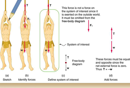
Figure 4.22 (a) A sketch of Tarzan hanging from a vine. (b) Arrows are used to represent all forces. T is the tension in the vine above Tarzan, FT is the force he exerts on the vine, and w is his weight. All other forces, such as the nudge of a breeze, are assumed negligible. (c) Suppose we are given the ape man’s mass and asked to find the
tension in the vine. We then define the system of interest as shown and draw a free-body diagram. FT is no longer shown, because it is not a force acting on the system of
interest; rather, FT acts on the outside world. (d) Showing only the arrows, the head-to-tail method of addition is used. It is apparent that T = - w , if Tarzan is stationary.
Step 2. Identify what needs to be determined and what is known or can be inferred from the problem as stated. That is, make a list of knowns and
unknowns. Then carefully determine the system of interest. This decision is a crucial step, since Newton’s second law involves only external forces.
Once the system of interest has been identified, it becomes possible to determine which forces are external and which are internal, a necessary step
to employ Newton’s second law. (See Figure 4.22(c).) Newton’s third law may be used to identify whether forces are exerted between components of
a system (internal) or between the system and something outside (external). As illustrated earlier in this chapter, the system of interest depends on
what question we need to answer. This choice becomes easier with practice, eventually developing into an almost unconscious process. Skill in
clearly defining systems will be beneficial in later chapters as well.
A diagram showing the system of interest and all of the external forces is called a free-body diagram. Only forces are shown on free-body diagrams,
not acceleration or velocity. We have drawn several of these in worked examples. Figure 4.22(c) shows a free-body diagram for the system of
interest. Note that no internal forces are shown in a free-body diagram.
Step 3. Once a free-body diagram is drawn, Newton’s second law can be applied to solve the problem. This is done in Figure 4.22(d) for a particular situation. In general, once external forces are clearly identified in free-body diagrams, it should be a straightforward task to put them into equation
form and solve for the unknown, as done in all previous examples. If the problem is one-dimensional—that is, if all forces are parallel—then they add
like scalars. If the problem is two-dimensional, then it must be broken down into a pair of one-dimensional problems. This is done by projecting the
force vectors onto a set of axes chosen for convenience. As seen in previous examples, the choice of axes can simplify the problem. For example,
when an incline is involved, a set of axes with one axis parallel to the incline and one perpendicular to it is most convenient. It is almost always
convenient to make one axis parallel to the direction of motion, if this is known.
Applying Newton’s Second Law
Before you write net force equations, it is critical to determine whether the system is accelerating in a particular direction. If the acceleration is
zero in a particular direction, then the net force is zero in that direction. Similarly, if the acceleration is nonzero in a particular direction, then the
net force is described by the equation: F net = ma .
For example, if the system is accelerating in the horizontal direction, but it is not accelerating in the vertical direction, then you will have the
following conclusions:
F
(4.56)
net x = ma,
CHAPTER 4 | DYNAMICS: FORCE AND NEWTON'S LAWS OF MOTION 143
F
(4.57)
net y = 0.
You will need this information in order to determine unknown forces acting in a system.
Step 4. As always, check the solution to see whether it is reasonable. In some cases, this is obvious. For example, it is reasonable to find that friction
causes an object to slide down an incline more slowly than when no friction exists. In practice, intuition develops gradually through problem solving,
and with experience it becomes progressively easier to judge whether an answer is reasonable. Another way to check your solution is to check the
units. If you are solving for force and end up with units of m/s, then you have made a mistake.
4.7 Further Applications of Newton’s Laws of Motion
There are many interesting applications of Newton’s laws of motion, a few more of which are presented in this section. These serve also to illustrate
some further subtleties of physics and to help build problem-solving skills.
Example 4.7 Drag Force on a Barge
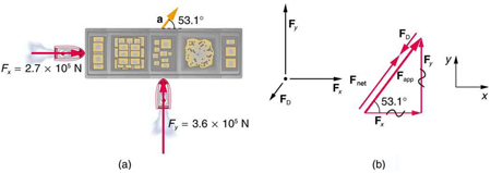
Suppose two tugboats push on a barge at different angles, as shown in Figure 4.23. The first tugboat exerts a force of 2.7×10⁵ N in the x-
direction, and the second tugboat exerts a force of 3.6×10⁵ N in the y-direction.
Figure 4.23 (a) A view from above of two tugboats pushing on a barge. (b) The free-body diagram for the ship contains only forces acting in the plane of the water. It
omits the two vertical forces—the weight of the barge and the buoyant force of the water supporting it cancel and are not shown. Since the applied forces are
perpendicular, the x- and y-axes are in the same direction as F x and F y . The problem quickly becomes a one-dimensional problem along the direction of Fapp , since friction is in the direction opposite to Fapp .
If the mass of the barge is 5.0×10⁶ kg and its acceleration is observed to be 7.5×10⁻² m/s2 in the direction shown, what is the drag force
of the water on the barge resisting the motion? (Note: drag force is a frictional force exerted by fluids, such as air or water. The drag force
opposes the motion of the object.)
Strategy
The directions and magnitudes of acceleration and the applied forces are given in Figure 4.23(a). We will define the total force of the tugboats on the barge as Fapp so that:
(4.58)
Fapp=F x + F y
Since the barge is flat bottomed, the drag of the water FD will be in the direction opposite to Fapp , as shown in the free-body diagram in
Figure 4.23(b). The system of interest here is the barge, since the forces on it are given as well as its acceleration. Our strategy is to find the magnitude and direction of the net applied force Fapp , and then apply Newton’s second law to solve for the drag force FD .
Solution
Since F x and F y are perpendicular, the magnitude and direction of Fapp are easily found. First, the resultant magnitude is given by the
Pythagorean theorem:
(4.59)
F
2
2
app =
F x + F y
F app = (2.7×10⁵ N)2 + (3.6×10⁵ N)2 = 4.5×10⁵ N.
The angle is given by
144 CHAPTER 4 | DYNAMICS: FORCE AND NEWTON'S LAWS OF MOTION
F
(4.60)
θ = tan−1⎛ y⎞
⎝ Fx⎠
θ = tan−1 ⎛3.6×10⁵ N⎞
⎝2.7×10⁵ N⎠ = 53º ,
which we know, because of Newton’s first law, is the same direction as the acceleration. FD is in the opposite direction of Fapp , since it acts to
slow down the acceleration. Therefore, the net external force is in the same direction as Fapp , but its magnitude is slightly less than Fapp . The
problem is now one-dimensional. From Figure 4.23(b), we can see that
F
(4.61)
net = F app − F D.
But Newton’s second law states that
F
(4.62)
net = ma.
Thus,
F
(4.63)
app − F D = ma.
This can be solved for the magnitude of the drag force of the water F D in terms of known quantities:
F
(4.64)
D = F app − ma.
Substituting known values gives
(4.65)
FD = (4.5×10⁵ N) − (5.0×10⁶ kg)(7.5×10⁻² m/s2) = 7.5×10⁴ N.
The direction of FD has already been determined to be in the direction opposite to Fapp , or at an angle of 53º south of west.
Discussion
The numbers used in this example are reasonable for a moderately large barge. It is certainly difficult to obtain larger accelerations with
tugboats, and small speeds are desirable to avoid running the barge into the docks. Drag is relatively small for a well-designed hull at low
speeds, consistent with the answer to this example, where F D is less than 1/600th of the weight of the ship.
In the earlier example of a tightrope walker we noted that the tensions in wires supporting a mass were equal only because the angles on either side
were equal. Consider the following example, where the angles are not equal; slightly more trigonometry is involved.
Example 4.8 Different Tensions at Different Angles
Consider the traffic light (mass 15.0 kg) suspended from two wires as shown in Figure 4.24. Find the tension in each wire, neglecting the
masses of the wires.
CHAPTER 4 | DYNAMICS: FORCE AND NEWTON'S LAWS OF MOTION 145
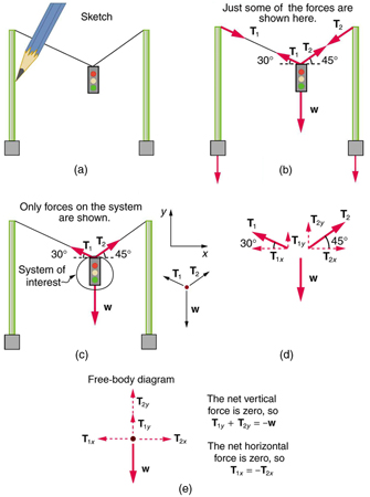
Figure 4.24 A traffic light is suspended from two wires. (b) Some of the forces involved. (c) Only forces acting on the system are shown here. The free-body diagram for
the traffic light is also shown. (d) The forces projected onto vertical ( y) and horizontal ( x) axes. The horizontal components of the tensions must cancel, and the sum of the vertical components of the tensions must equal the weight of the traffic light. (e) The free-body diagram shows the vertical and horizontal forces acting on the traffic light.
Strategy
The system of interest is the traffic light, and its free-body diagram is shown in Figure 4.24(c). The three forces involved are not parallel, and so
they must be projected onto a coordinate system. The most convenient coordinate system has one axis vertical and one horizontal, and the
vector projections on it are shown in part (d) of the figure. There are two unknowns in this problem ( T 1 and T 2 ), so two equations are needed
to find them. These two equations come from applying Newton’s second law along the vertical and horizontal axes, noting that the net external
force is zero along each axis because acceleration is zero.
Solution
First consider the horizontal or x-axis:
F
(4.66)
net x = T 2 x − T 1 x = 0.
Thus, as you might expect,
T
(4.67)
1 x = T 2 x.
This gives us the following relationship between T 1 and T 2 :
T
(4.68)
1 cos (30º) = T 2 cos (45º).
Thus,
T
(4.69)
2 = (1.225) T 1.
Note that T 1 and T 2 are not equal in this case, because the angles on either side are not equal. It is reasonable that T 2 ends up being
greater than T 1 , because it is exerted more vertically than T 1 .
Now consider the force components along the vertical or y-axis:
F
(4.70)
net y = T 1 y + T 2 y − w = 0.
146 CHAPTER 4 | DYNAMICS: FORCE AND NEWTON'S LAWS OF MOTION
This implies
T
(4.71)
1 y + T 2 y = w.
Substituting the expressions for the vertical components gives
T
(4.72)
1 sin (30º) + T 2 sin (45º) = w.
There are two unknowns in this equation, but substituting the expression for T 2 in terms of T 1 reduces this to one equation with one unknown:
T
(4.73)
1(0.500) + (1.225 T 1)(0.707) = w = mg,
which yields
(4.74)
(1.366) T 1 = (15.0 kg)(9.80 m/s2).
Solving this last equation gives the magnitude of T 1 to be
T
(4.75)
1 = 108 N.
Finally, the magnitude of T 2 is determined using the relationship between them, T 2 = 1.225 T 1 , found above. Thus we obtain
T
(4.76)
2 = 132 N.
Discussion
Both tensions would be larger if both wires were more horizontal, and they will be equal if and only if the angles on either side are the same (as
they were in the earlier example of a tightrope walker).
The bathroom scale is an excellent example of a normal force acting on a body. It provides a quantitative reading of how much it must push upward
to support the weight of an object. But can you predict what you would see on the dial of a bathroom scale if you stood on it during an elevator ride?
Will you see a value greater than your weight when the elevator starts up? What about when the elevator moves upward at a constant speed: will the
scale still read more than your weight at rest? Consider the following example.
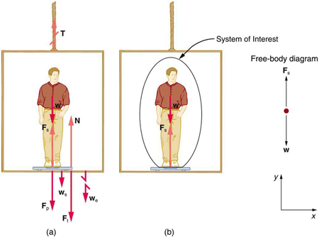
Example 4.9 What Does the Bathroom Scale Read in an Elevator?
Figure 4.25 shows a 75.0-kg man (weight of about 165 lb) standing on a bathroom scale in an elevator. Calculate the scale reading: (a) if the
elevator accelerates upward at a rate of 1.20 m/s2 , and (b) if the elevator moves upward at a constant speed of 1 m/s.
Figure 4.25 (a)