0.70
Bicycle
0.90
Skydiver (horizontal) 1.0
Circular flat plate
1.12
Substantial research is under way in the sporting world to minimize drag. The dimples on golf balls are being redesigned as are the clothes that
athletes wear. Bicycle racers and some swimmers and runners wear full bodysuits. Australian Cathy Freeman wore a full body suit in the 2000
Sydney Olympics, and won the gold medal for the 400 m race. Many swimmers in the 2008 Beijing Olympics wore (Speedo) body suits; it might have
made a difference in breaking many world records (See Figure 5.10). Most elite swimmers (and cyclists) shave their body hair. Such innovations can
have the effect of slicing away milliseconds in a race, sometimes making the difference between a gold and a silver medal. One consequence is that
careful and precise guidelines must be continuously developed to maintain the integrity of the sport.
Figure 5.10 Body suits, such as this LZR Racer Suit, have been credited with many world records after their release in 2008. Smoother “skin” and more compression forces on
a swimmer’s body provide at least 10% less drag. (credit: NASA/Kathy Barnstorff)
Some interesting situations connected to Newton’s second law occur when considering the effects of drag forces upon a moving object. For instance,
consider a skydiver falling through air under the influence of gravity. The two forces acting on him are the force of gravity and the drag force (ignoring
the buoyant force). The downward force of gravity remains constant regardless of the velocity at which the person is moving. However, as the
person’s velocity increases, the magnitude of the drag force increases until the magnitude of the drag force is equal to the gravitational force, thus
producing a net force of zero. A zero net force means that there is no acceleration, as given by Newton’s second law. At this point, the person’s
velocity remains constant and we say that the person has reached his terminal velocity ( v t ). Since F D is proportional to the speed, a heavier
skydiver must go faster for F D to equal his weight. Let’s see how this works out more quantitatively.
At the terminal velocity,
F
(5.16)
net = mg − F D = ma = 0.
Thus,
mg
(5.17)
= F D.
Using the equation for drag force, we have
(5.18)
mg = 12 ρCAv 2.
Solving for the velocity, we obtain
CHAPTER 5 | FURTHER APPLICATIONS OF NEWTON'S LAWS: FRICTION, DRAG, AND ELASTICITY 169
(5.19)
v = 2 mg
ρCA.
Assume the density of air is ρ = 1.21 kg/m3 . A 75-kg skydiver descending head first will have an area approximately A = 0.18 m2 and a drag
coefficient of approximately C = 0.70 . We find that
(5.20)
v =
2(75 kg)(9.80 m/s2)
(1.21 kg/m3)(0.70)(0.18 m2)
= 98 m/s
= 350 km/h.
This means a skydiver with a mass of 75 kg achieves a maximum terminal velocity of about 350 km/h while traveling in a pike (head first) position,
minimizing the area and his drag. In a spread-eagle position, that terminal velocity may decrease to about 200 km/h as the area increases. This
terminal velocity becomes much smaller after the parachute opens.
Take-Home Experiment
This interesting activity examines the effect of weight upon terminal velocity. Gather together some nested coffee filters. Leaving them in their
original shape, measure the time it takes for one, two, three, four, and five nested filters to fall to the floor from the same height (roughly 2 m).
(Note that, due to the way the filters are nested, drag is constant and only mass varies.) They obtain terminal velocity quite quickly, so find this
velocity as a function of mass. Plot the terminal velocity v versus mass. Also plot v2 versus mass. Which of these relationships is more linear?
What can you conclude from these graphs?
Example 5.2 A Terminal Velocity
Find the terminal velocity of an 85-kg skydiver falling in a spread-eagle position.
Strategy
At terminal velocity, F net = 0 . Thus the drag force on the skydiver must equal the force of gravity (the person’s weight). Using the equation of
drag force, we find mg = 12 ρCAv 2 .
Thus the terminal velocity v t can be written as
(5.21)
v t = 2 mg
ρCA.
Solution
All quantities are known except the person’s projected area. This is an adult (82 kg) falling spread eagle. We can estimate the frontal area as
(5.22)
A = (2 m)(0.35 m) = 0.70 m2.
Using our equation for v t , we find that
(5.23)
v t =
2(85 kg)(9.80 m/s2)
(1.21 kg/m3)(1.0)(0.70 m2)
= 44 m/s.
Discussion
This result is consistent with the value for v t mentioned earlier. The 75-kg skydiver going feet first had a v = 98 m / s . He weighed less but
had a smaller frontal area and so a smaller drag due to the air.
The size of the object that is falling through air presents another interesting application of air drag. If you fall from a 5-m high branch of a tree, you will
likely get hurt—possibly fracturing a bone. However, a small squirrel does this all the time, without getting hurt. You don’t reach a terminal velocity in
such a short distance, but the squirrel does.
The following interesting quote on animal size and terminal velocity is from a 1928 essay by a British biologist, J.B.S. Haldane, titled “On Being the
Right Size.”
To the mouse and any smaller animal, [gravity] presents practically no dangers. You can drop a mouse down a thousand-yard mine shaft; and, on
arriving at the bottom, it gets a slight shock and walks away, provided that the ground is fairly soft. A rat is killed, a man is broken, and a horse
splashes. For the resistance presented to movement by the air is proportional to the surface of the moving object. Divide an animal’s length, breadth,
and height each by ten; its weight is reduced to a thousandth, but its surface only to a hundredth. So the resistance to falling in the case of the small
animal is relatively ten times greater than the driving force.
The above quadratic dependence of air drag upon velocity does not hold if the object is very small, is going very slow, or is in a denser medium than
air. Then we find that the drag force is proportional just to the velocity. This relationship is given by Stokes’ law, which states that

170 CHAPTER 5 | FURTHER APPLICATIONS OF NEWTON'S LAWS: FRICTION, DRAG, AND ELASTICITY
F
(5.24)
s = 6 πrηv,
where r is the radius of the object, η is the viscosity of the fluid, and v is the object’s velocity.
Stokes’ Law
F
(5.25)
s = 6 πrηv,
where r is the radius of the object, η is the viscosity of the fluid, and v is the object’s velocity.
Good examples of this law are provided by microorganisms, pollen, and dust particles. Because each of these objects is so small, we find that many
of these objects travel unaided only at a constant (terminal) velocity. Terminal velocities for bacteria (size about 1 μm ) can be about 2 μm/s . To
move at a greater speed, many bacteria swim using flagella (organelles shaped like little tails) that are powered by little motors embedded in the cell.
Sediment in a lake can move at a greater terminal velocity (about 5 μm/s ), so it can take days to reach the bottom of the lake after being deposited
on the surface.
If we compare animals living on land with those in water, you can see how drag has influenced evolution. Fishes, dolphins, and even massive whales
are streamlined in shape to reduce drag forces. Birds are streamlined and migratory species that fly large distances often have particular features
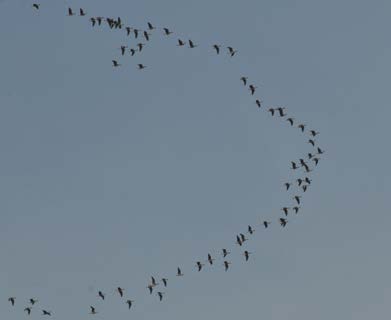
such as long necks. Flocks of birds fly in the shape of a spear head as the flock forms a streamlined pattern (see Figure 5.11). In humans, one
important example of streamlining is the shape of sperm, which need to be efficient in their use of energy.
Figure 5.11 Geese fly in a V formation during their long migratory travels. This shape reduces drag and energy consumption for individual birds, and also allows them a better
way to communicate. (credit: Julo, Wikimedia Commons)
Galileo’s Experiment
Galileo is said to have dropped two objects of different masses from the Tower of Pisa. He measured how long it took each to reach the ground.
Since stopwatches weren’t readily available, how do you think he measured their fall time? If the objects were the same size, but with different
masses, what do you think he should have observed? Would this result be different if done on the Moon?
PhET Explorations: Masses & Springs
A realistic mass and spring laboratory. Hang masses from springs and adjust the spring stiffness and damping. You can even slow time.
Transport the lab to different planets. A chart shows the kinetic, potential, and thermal energy for each spring.
Figure 5.12 Masses & Springs (http://cnx.org/content/m42080/1.4/mass-spring-lab_en.jar)
5.3 Elasticity: Stress and Strain
We now move from consideration of forces that affect the motion of an object (such as friction and drag) to those that affect an object’s shape. If a
bulldozer pushes a car into a wall, the car will not move but it will noticeably change shape. A change in shape due to the application of a force is a
deformation. Even very small forces are known to cause some deformation. For small deformations, two important characteristics are observed.
First, the object returns to its original shape when the force is removed—that is, the deformation is elastic for small deformations. Second, the size of
the deformation is proportional to the force—that is, for small deformations, Hooke’s law is obeyed. In equation form, Hooke’s law is given by
F
(5.26)
= kΔ L,
CHAPTER 5 | FURTHER APPLICATIONS OF NEWTON'S LAWS: FRICTION, DRAG, AND ELASTICITY 171
where Δ L is the amount of deformation (the change in length, for example) produced by the force F , and k is a proportionality constant that
depends on the shape and composition of the object and the direction of the force. Note that this force is a function of the deformation Δ L —it is not
constant as a kinetic friction force is. Rearranging this to
(5.27)
Δ L = Fk
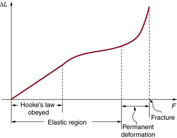
makes it clear that the deformation is proportional to the applied force. Figure 5.13 shows the Hooke’s law relationship between the extension Δ L of a spring or of a human bone. For metals or springs, the straight line region in which Hooke’s law pertains is much larger. Bones are brittle and the
elastic region is small and the fracture abrupt. Eventually a large enough stress to the material will cause it to break or fracture.
Hooke’s Law
F
(5.28)
= kΔL,
where Δ L is the amount of deformation (the change in length, for example) produced by the force F , and k is a proportionality constant that
depends on the shape and composition of the object and the direction of the force.
(5.29)
Δ L = Fk
Figure 5.13 A graph of deformation Δ L versus applied force F . The straight segment is the linear region where Hooke’s law is obeyed. The slope of the straight region is 1 k . For larger forces, the graph is curved but the deformation is still elastic— Δ L will return to zero if the force is removed. Still greater forces permanently deform the object until it finally fractures. The shape of the curve near fracture depends on several factors, including how the force F is applied. Note that in this graph the slope increases just before fracture, indicating that a small increase in F is producing a large increase in L near the fracture.
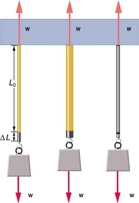
The proportionality constant k depends upon a number of factors for the material. For example, a guitar string made of nylon stretches when it is
tightened, and the elongation Δ L is proportional to the force applied (at least for small deformations). Thicker nylon strings and ones made of steel
stretch less for the same applied force, implying they have a larger k (see Figure 5.14). Finally, all three strings return to their normal lengths when the force is removed, provided the deformation is small. Most materials will behave in this manner if the deformation is less that about 0.1% or about
1 part in 103 .
Figure 5.14 The same force, in this case a weight ( w ), applied to three different guitar strings of identical length produces the three different deformations shown as shaded segments. The string on the left is thin nylon, the one in the middle is thicker nylon, and the one on the right is steel.
172 CHAPTER 5 | FURTHER APPLICATIONS OF NEWTON'S LAWS: FRICTION, DRAG, AND ELASTICITY
Stretch Yourself a Little
How would you go about measuring the proportionality constant k of a rubber band? If a rubber band stretched 3 cm when a 100-g mass was
attached to it, then how much would it stretch if two similar rubber bands were attached to the same mass—even if put together in parallel or
alternatively if tied together in series?
We now consider three specific types of deformations: changes in length (tension and compression), sideways shear (stress), and changes in
volume. All deformations are assumed to be small unless otherwise stated.
Changes in Length—Tension and Compression: Elastic Modulus
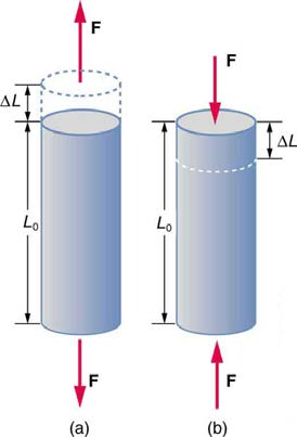
A change in length Δ L is produced when a force is applied to a wire or rod parallel to its length L 0 , either stretching it (a tension) or compressing it.
(See Figure 5.15.)
Figure 5.15 (a) Tension. The rod is stretched a length Δ L when a force is applied parallel to its length. (b) Compression. The same rod is compressed by forces with the same magnitude in the opposite direction. For very small deformations and uniform materials, Δ L is approximately the same for the same magnitude of tension or
compression. For larger deformations, the cross-sectional area changes as the rod is compressed or stretched.
Experiments have shown that the change in length ( Δ L ) depends on only a few variables. As already noted, Δ L is proportional to the force F and
depends on the substance from which the object is made. Additionally, the change in length is proportional to the original length L 0 and inversely
proportional to the cross-sectional area of the wire or rod. For example, a long guitar string will stretch more than a short one, and a thick string will
stretch less than a thin one. We can combine all these factors into one equation for Δ L :
F
(5.30)
Δ L = 1 Y AL 0,
where Δ L is the change in length, F the applied force, Y is a factor, called the elastic modulus or Young’s modulus, that depends on the
substance, A is the cross-sectional area, and L 0 is the original length. Table 5.3 lists values of Y for several materials—those with a large Y are said to have a large tensile strength because they deform less for a given tension or compression.

CHAPTER 5 | FURTHER APPLICATIONS OF NEWTON'S LAWS: FRICTION, DRAG, AND ELASTICITY 173
Table 5.3 Elastic Moduli[1]
Young’s modulus (tension–compression) Y
Shear modulus S
Bulk modulus B
Material
(109 N/m2)
(109 N/m2)
(109 N/m2)
Aluminum
70
25
75
Bone – tension
16
80
8
Bone –
9
compression
Brass
90
35
75
Brick
15
Concrete
20
Glass
70
20
30
Granite
45
20
45
Hair (human)
10
Hardwood
15
10
Iron, cast
100
40
90
Lead
16
5
50
Marble
60
20
70
Nylon
5
Polystyrene
3
Silk
6
Spider thread
3
Steel
210
80
130
Tendon
1
Acetone
0.7
Ethanol
0.9
Glycerin
4.5
Mercury
25
Water
2.2
Young’s moduli are not listed for liquids and gases in Table 5.3 because they cannot be stretched or compressed in only one direction. Note that
there is an assumption that the object does not accelerate, so that there are actually two applied forces of magnitude F acting in opposite directions.
For example, the strings in Figure 5.15 are being pulled down by a force of magnitude w and held up by the ceiling, which also exerts a force of magnitude w .
Example 5.3 The Stretch of a Long Cable
Suspension cables are used to carry gondolas at ski resorts. (See Figure 5.16) Consider a suspension cable that includes an unsupported span
of 3 km. Calculate the amount of stretch in the steel cable. Assume that the cable has a diameter of 5.6 cm and the maximum tension it can
withstand is 3.0×10⁶ N .
Figure 5.16 Gondolas travel along suspension cables at the Gala Yuzawa ski resort in Japan. (credit: Rudy Herman, Flickr)
Strategy
1. Approximate and average values. Young’s moduli Y for tension and compression sometimes differ but are averaged here. Bone has significantly
different Young’s moduli for tension and compression.
174 CHAPTER 5 | FURTHER APPLICATIONS OF NEWTON'S LAWS: FRICTION, DRAG, AND ELASTICITY
The force is equal to the maximum tension, or F = 3.0×10⁶ N . The cross-sectional area is πr 2 = 2.46×10⁻³ m2 . The equation
Δ L = 1 F
Y AL 0 can be used to find the change in length.
Solution
All quantities are known. Thus,
(5.31)
Δ L = ⎛
⎞⎛ 3.0×10⁶ N ⎞
⎝
1
210×109 N/m2⎠⎝2.46×10–3 m2⎠(3020 m)
= 18 m.
Discussion
This is quite a stretch, but only about 0.6% of the unsupported length. Effects of temperature upon length might be important in these
environments.
Bones, on the whole, do not fracture due to tension or compression. Rather they generally fracture due to sideways impact or bending, resulting in
the bone shearing or snapping. The behavior of bones under tension and compression is important because it determines the load the bones can
carry. Bones are classified as weight-bearing structures such as columns in buildings and trees. Weight-bearing structures have special features;
columns in building have steel-reinforcing rods while trees and bones are fibrous. The bones in different parts of the body serve different structural
functions and are prone to different stresses. Thus the bone in the top of the femur is arranged in thin sheets separated by marrow while in other
places the bones can be cylindrical and filled with marrow or just solid. Overweight people have a tendency toward bone damage due to sustained
compressions in bone joints and tendons.
Another biological example of Hooke’s law occurs in tendons. Functionally, the tendon (the tissue connecting muscle to bone) must stretch easily at
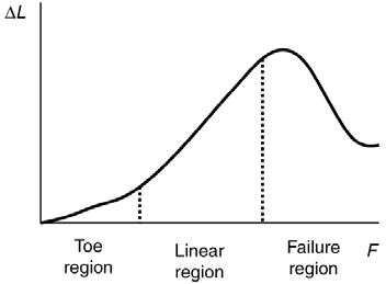
first when a force is applied, but offer a much greater restoring force for a greater strain. Figure 5.17 shows a stress-strain relationship for a human tendon. Some tendons have a high collagen content so there is relatively little strain, or length change; others, like support tendons (as in the leg) can
change length up to 10%. Note that this stress-strain curve is nonlinear, since the slope of the line changes in different regions. In the first part of the
stretch called the toe region, the fibers in the tendon begin to align in the direction of the stress—this is called uncrimping. In the linear region, the
fibrils will be stretched, and in the failure region individual fibers begin to break. A simple model of this relationship can be illustrated by springs in
parallel: different springs are activated at different lengths of stretch. Examples of this are given in the problems at end of this chapter. Ligaments
(tissue connecting bone to bone) behave in a similar way.
Figure 5.17 Typical stress-strain curve for mammalian tendon. Three regions are shown: (1) toe region (2) linear region, and (3) failure region.
Unlike bones and tendons, which need to be strong as well as elastic, the arteries and lungs need to be very stretchable. The elastic properties of the
arteries are essential for blood flow. The pressure in the arteries increases and arterial walls stretch when the blood is pumped out of the heart. When
the aortic valve shuts, the pressure in the arteries drops and the arterial walls relax to maintain the blood flow. When you feel your pulse, you are
feeling exactly this—the elastic behavior of the arteries as the blood gushes through with each pump of the heart. If the arteries were rigid, you would
not feel a pulse. The heart is also an organ with special elastic properties. The lungs expand with muscular effort when we breathe in but relax freely
and elastically when we breathe out. Our skins are particularly elastic, especially for the young. A young person can go from 100 kg to 60 kg with no
visible sag in their skins. The elasticity of all organs reduces with age. Gradual physiological aging through reduction in elasticity starts in the early
20s.
Example 5.4 Calculating Deformation: How Much Does Your Leg Shorten When You Stand on It?
Calculate the change in length of the upper leg bone (the femur) when a 70.0 kg man supports 62.0 kg of his mass on it, assuming the bone to
be equivalent to a uniform rod that is 40.0 cm long and 2.00 cm in radius.
Strategy
The force is equal to the weight supported, or
⎛