There is more to motion than distance and displacement. Questions such as, “How long does a foot race take?” and “What was the runner’s speed?”
cannot be answered without an understanding of other concepts. In this section we add definitions of time, velocity, and speed to expand our
description of motion.
Time
As discussed in Physical Quantities and Units, the most fundamental physical quantities are defined by how they are measured. This is the case
with time. Every measurement of time involves measuring a change in some physical quantity. It may be a number on a digital clock, a heartbeat, or
the position of the Sun in the sky. In physics, the definition of time is simple— time is change, or the interval over which change occurs. It is
impossible to know that time has passed unless something changes.
The amount of time or change is calibrated by comparison with a standard. The SI unit for time is the second, abbreviated s. We might, for example,
observe that a certain pendulum makes one full swing every 0.75 s. We could then use the pendulum to measure time by counting its swings or, of
course, by connecting the pendulum to a clock mechanism that registers time on a dial. This allows us to not only measure the amount of time, but
also to determine a sequence of events.
How does time relate to motion? We are usually interested in elapsed time for a particular motion, such as how long it takes an airplane passenger to
get from his seat to the back of the plane. To find elapsed time, we note the time at the beginning and end of the motion and subtract the two. For
40 CHAPTER 2 | KINEMATICS
example, a lecture may start at 11:00 A.M. and end at 11:50 A.M., so that the elapsed time would be 50 min. Elapsed time Δ t is the difference
between the ending time and beginning time,
(2.4)
Δ t = t f − t 0,
where Δ t is the change in time or elapsed time, t f is the time at the end of the motion, and t 0 is the time at the beginning of the motion. (As usual,
the delta symbol, Δ , means the change in the quantity that follows it.)
Life is simpler if the beginning time t 0 is taken to be zero, as when we use a stopwatch. If we were using a stopwatch, it would simply read zero at
the start of the lecture and 50 min at the end. If t 0 = 0 , then Δ t = t f ≡ t .
In this text, for simplicity’s sake,
• motion starts at time equal to zero ( t 0 = 0)
• the symbol t is used for elapsed time unless otherwise specified (Δ t = t f ≡ t)
Velocity
Your notion of velocity is probably the same as its scientific definition. You know that if you have a large displacement in a small amount of time you
have a large velocity, and that velocity has units of distance divided by time, such as miles per hour or kilometers per hour.
Average Velocity
Average velocity is displacement (change in position) divided by the time of travel,
(2.5)
v- = Δ x
Δ t = x f − x 0
t
,
f − t 0
where v- is the average (indicated by the bar over the v ) velocity, Δ x is the change in position (or displacement), and x f and x 0 are the final and beginning positions at times t f and t 0 , respectively. If the starting time t 0 is taken to be zero, then the average velocity is simply
(2.6)
v- = Δ x
t .
Notice that this definition indicates that velocity is a vector because displacement is a vector. It has both magnitude and direction. The SI unit for
velocity is meters per second or m/s, but many other units, such as km/h, mi/h (also written as mph), and cm/s, are in common use. Suppose, for
example, an airplane passenger took 5 seconds to move −4 m (the negative sign indicates that displacement is toward the back of the plane). His
average velocity would be
(2.7)
v- = Δ x
t = −4 m
5 s = − 0.8 m/s.
The minus sign indicates the average velocity is also toward the rear of the plane.
The average velocity of an object does not tell us anything about what happens to it between the starting point and ending point, however. For
example, we cannot tell from average velocity whether the airplane passenger stops momentarily or backs up before he goes to the back of the
plane. To get more details, we must consider smaller segments of the trip over smaller time intervals.
Figure 2.9 A more detailed record of an airplane passenger heading toward the back of the plane, showing smaller segments of his trip.
The smaller the time intervals considered in a motion, the more detailed the information. When we carry this process to its logical conclusion, we are
left with an infinitesimally small interval. Over such an interval, the average velocity becomes the instantaneous velocity or the velocity at a specific
instant. A car’s speedometer, for example, shows the magnitude (but not the direction) of the instantaneous velocity of the car. (Police give tickets
based on instantaneous velocity, but when calculating how long it will take to get from one place to another on a road trip, you need to use average
velocity.) Instantaneous velocity v is the average velocity at a specific instant in time (or over an infinitesimally small time interval).
Mathematically, finding instantaneous velocity, v , at a precise instant t can involve taking a limit, a calculus operation beyond the scope of this text.
However, under many circumstances, we can find precise values for instantaneous velocity without calculus.
CHAPTER 2 | KINEMATICS 41
Speed
In everyday language, most people use the terms “speed” and “velocity” interchangeably. In physics, however, they do not have the same meaning
and they are distinct concepts. One major difference is that speed has no direction. Thus speed is a scalar. Just as we need to distinguish between
instantaneous velocity and average velocity, we also need to distinguish between instantaneous speed and average speed.
Instantaneous speed is the magnitude of instantaneous velocity. For example, suppose the airplane passenger at one instant had an instantaneous
velocity of −3.0 m/s (the minus meaning toward the rear of the plane). At that same time his instantaneous speed was 3.0 m/s. Or suppose that at
one time during a shopping trip your instantaneous velocity is 40 km/h due north. Your instantaneous speed at that instant would be 40 km/h—the
same magnitude but without a direction. Average speed, however, is very different from average velocity. Average speed is the distance traveled
divided by elapsed time.
We have noted that distance traveled can be greater than displacement. So average speed can be greater than average velocity, which is
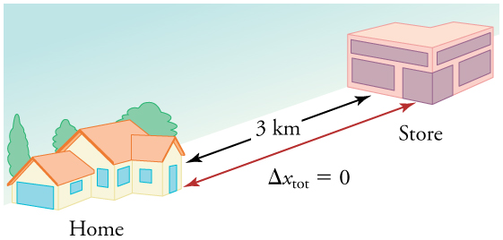
displacement divided by time. For example, if you drive to a store and return home in half an hour, and your car’s odometer shows the total distance
traveled was 6 km, then your average speed was 12 km/h. Your average velocity, however, was zero, because your displacement for the round trip is
zero. (Displacement is change in position and, thus, is zero for a round trip.) Thus average speed is not simply the magnitude of average velocity.
Figure 2.10 During a 30-minute round trip to the store, the total distance traveled is 6 km. The average speed is 12 km/h. The displacement for the round trip is zero, since
there was no net change in position. Thus the average velocity is zero.
Another way of visualizing the motion of an object is to use a graph. A plot of position or of velocity as a function of time can be very useful. For
example, for this trip to the store, the position, velocity, and speed-vs.-time graphs are displayed in Figure 2.11. (Note that these graphs depict a very
simplified model of the trip. We are assuming that speed is constant during the trip, which is unrealistic given that we’ll probably stop at the store. But
for simplicity’s sake, we will model it with no stops or changes in speed. We are also assuming that the route between the store and the house is a
perfectly straight line.)
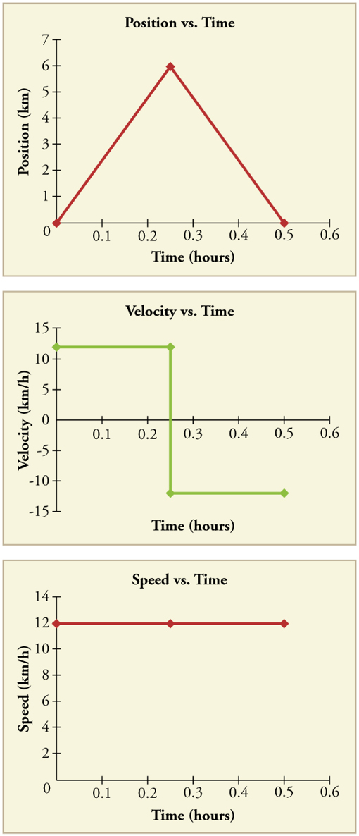
42 CHAPTER 2 | KINEMATICS
Figure 2.11 Position vs. time, velocity vs. time, and speed vs. time on a trip. Note that the velocity for the return trip is negative.
Making Connections: Take-Home Investigation—Getting a Sense of Speed
If you have spent much time driving, you probably have a good sense of speeds between about 10 and 70 miles per hour. But what are these in
meters per second? What do we mean when we say that something is moving at 10 m/s? To get a better sense of what these values really
mean, do some observations and calculations on your own:
• calculate typical car speeds in meters per second
• estimate jogging and walking speed by timing yourself; convert the measurements into both m/s and mi/h
• determine the speed of an ant, snail, or falling leaf
A commuter train travels from Baltimore to Washington, DC, and back in 1 hour and 45 minutes. The distance between the two stations is
approximately 40 miles. What is (a) the average velocity of the train, and (b) the average speed of the train in m/s?
Solution

CHAPTER 2 | KINEMATICS 43
(a) The average velocity of the train is zero because x f = x 0 ; the train ends up at the same place it starts.
(b) The average speed of the train is calculated below. Note that the train travels 40 miles one way and 40 miles back, for a total distance of 80
miles.
(2.8)
distance
time = 80 miles
105 minutes
(2.9)
80 miles
105 minutes×5280 feet
1 mile × 1 meter
3.28 feet× 1 minute
60 seconds = 20 m/s
2.4 Acceleration
Figure 2.12 A plane decelerates, or slows down, as it comes in for landing in St. Maarten. Its acceleration is opposite in direction to its velocity. (credit: Steve Conry, Flickr) In everyday conversation, to accelerate means to speed up. The accelerator in a car can in fact cause it to speed up. The greater the acceleration,
the greater the change in velocity over a given time. The formal definition of acceleration is consistent with these notions, but more inclusive.
Average Acceleration
Average Acceleration is the rate at which velocity changes,
(2.10)
a- = Δ v
Δ t = v f − v 0
t
,
f − t 0
where a- is average acceleration, v is velocity, and t is time. (The bar over the a means average acceleration.)
Because acceleration is velocity in m/s divided by time in s, the SI units for acceleration are m/s2 , meters per second squared or meters per second
per second, which literally means by how many meters per second the velocity changes every second.
Recall that velocity is a vector—it has both magnitude and direction. This means that a change in velocity can be a change in magnitude (or speed),
but it can also be a change in direction. For example, if a car turns a corner at constant speed, it is accelerating because its direction is changing. The
quicker you turn, the greater the acceleration. So there is an acceleration when velocity changes either in magnitude (an increase or decrease in
speed) or in direction, or both.
Acceleration as a Vector
Acceleration is a vector in the same direction as the change in velocity, Δ v . Since velocity is a vector, it can change either in magnitude or in
direction. Acceleration is therefore a change in either speed or direction, or both.
Keep in mind that although acceleration is in the direction of the change in velocity, it is not always in the direction of motion. When an object slows
down, its acceleration is opposite to the direction of its motion. This is known as deceleration.
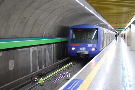
44 CHAPTER 2 | KINEMATICS
Figure 2.13 A subway train in Sao Paulo, Brazil, decelerates as it comes into a station. It is accelerating in a direction opposite to its direction of motion. (credit: Yusuke
Kawasaki, Flickr)
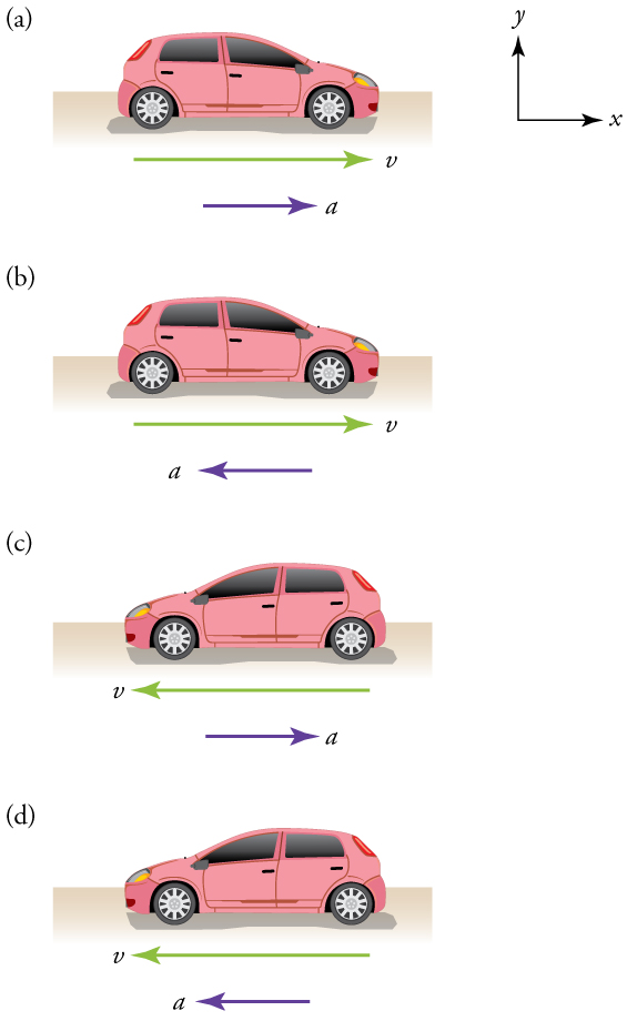
Misconception Alert: Deceleration vs. Negative Acceleration
Deceleration always refers to acceleration in the direction opposite to the direction of the velocity. Deceleration always reduces speed. Negative
acceleration, however, is acceleration in the negative direction in the chosen coordinate system. Negative acceleration may or may not be
deceleration, and deceleration may or may not be considered negative acceleration. For example, consider Figure 2.14.
Figure 2.14 (a) This car is speeding up as it moves toward the right. It therefore has positive acceleration in our coordinate system. (b) This car is slowing down as it
moves toward the right. Therefore, it has negative acceleration in our coordinate system, because its acceleration is toward the left. The car is also decelerating: the
direction of its acceleration is opposite to its direction of motion. (c) This car is moving toward the left, but slowing down over time. Therefore, its acceleration is positive in
our coordinate system because it is toward the right. However, the car is decelerating because its acceleration is opposite to its motion. (d) This car is speeding up as it
moves toward the left. It has negative acceleration because it is accelerating toward the left. However, because its acceleration is in the same direction as its motion, it is
speeding up ( not decelerating).
CHAPTER 2 | KINEMATICS 45
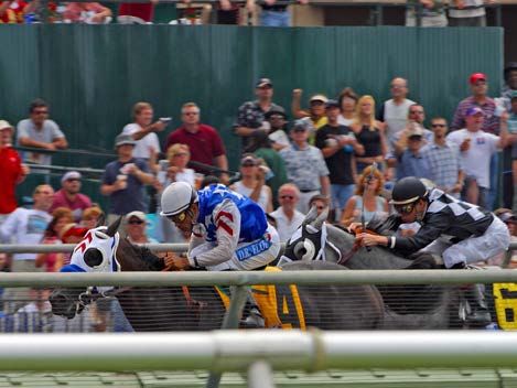
Example 2.1 Calculating Acceleration: A Racehorse Leaves the Gate
A racehorse coming out of the gate accelerates from rest to a velocity of 15.0 m/s due west in 1.80 s. What is its average acceleration?
Figure 2.15 (credit: Jon Sullivan, PD Photo.org)
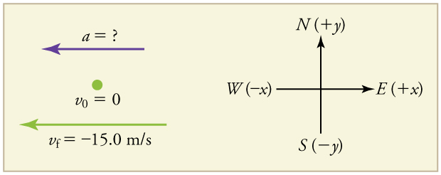
Strategy
First we draw a sketch and assign a coordinate system to the problem. This is a simple problem, but it always helps to visualize it. Notice that we
assign east as positive and west as negative. Thus, in this case, we have negative velocity.
Figure 2.16
We can solve this problem by identifying Δ v and Δ t from the given information and then calculating the average acceleration directly from the
equation a- = Δ v
Δ t = v f − v 0
t
.
f − t 0
Solution
1. Identify the knowns. v 0 = 0 , v f = −15.0 m/s (the negative sign indicates direction toward the west), Δ t = 1.80 s .
2. Find the change in velocity. Since the horse is going from zero to − 15.0 m/s , its change in velocity equals its final velocity:
Δ v = v f = −15.0 m/s .
3. Plug in the known values ( Δ v and Δ t ) and solve for the unknown a- .
(2.11)
a- = Δ v
Δ t = −15.0 m/s
1.80 s = −8.33 m/s2.
Discussion
The negative sign for acceleration indicates that acceleration is toward the west. An acceleration of 8.33 m/s2 due west means that the horse
increases its velocity by 8.33 m/s due west each second, that is, 8.33 meters per second per second, which we write as 8.33 m/s2 . This is truly
an average acceleration, because the ride is not smooth. We shall see later that an acceleration of this magnitude would require the rider to hang
on with a force nearly equal to his weight.
Instantaneous Acceleration
Instantaneous acceleration a , or the acceleration at a specific instant in time, is obtained by the same process as discussed for instantaneous
using only algebra? The answer is that we choose an average acceleration that is representative of the motion. Figure 2.17 shows graphs of
instantaneous acceleration versus time for two very different motions. In Figure 2.17(a), the acceleration varies slightly and the average over the
entire interval is nearly the same as the instantaneous acceleration at any time. In this case, we should treat this motion as if it had a constant
acceleration equal to the average (in this case about 1.8 m/s2 ). In Figure 2.17(b), the acceleration varies drastically over time. In such situations it
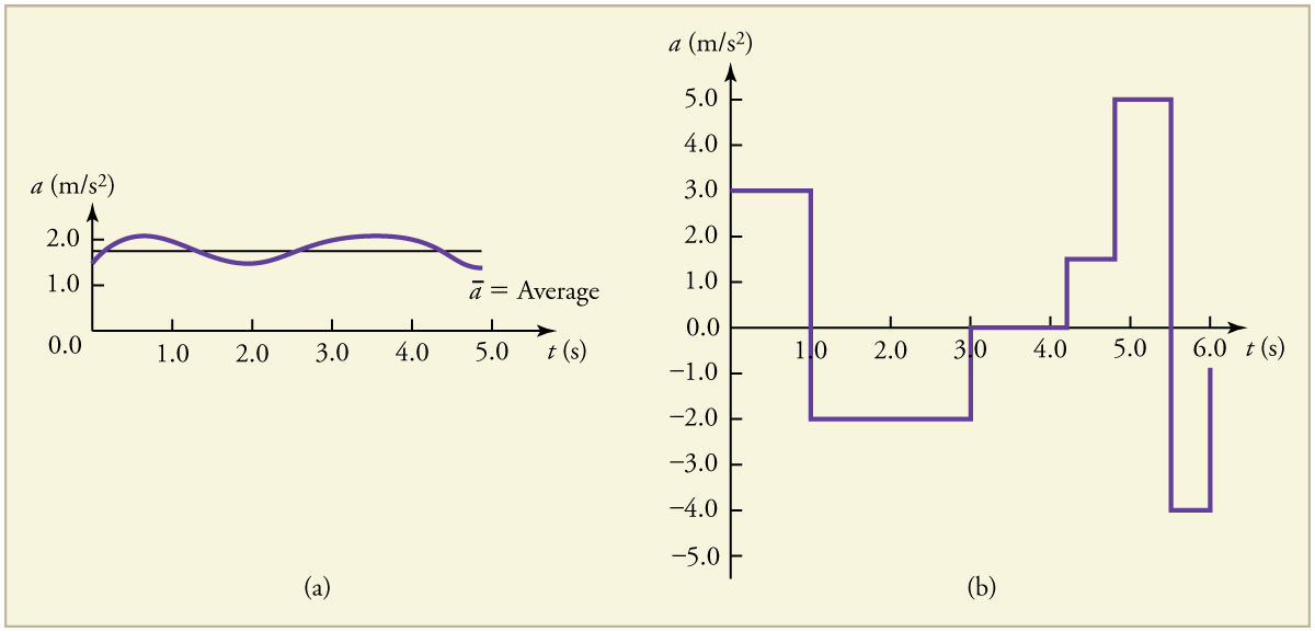
46 CHAPTER 2 | KINEMATICS
is best to consider smaller time intervals and choose an average acceleration for each. For example, we could consider motion over the time intervals
from 0 to 1.0 s and from 1.0 to 3.0 s as separate motions with accelerations of +3.0 m/s2 and –2.0 m/s2 , respectively.
Figure 2.17 Graphs of instantaneous acceleration versus time for two different one-dimensional motions. (a) Here acceleration varies only slightly and is always in the same
direction, since it is positive. The average over the interval is nearly the same as the acceleration at any given time. (b) Here the acceleration varies greatly, perhaps
representing a package on a post office conveyor belt that is accelerated forward and backward as it bumps along. It is necessary to consider small time intervals (such as
from 0 to 1.0 s) with constant or nearly constant acceleration in such a situation.
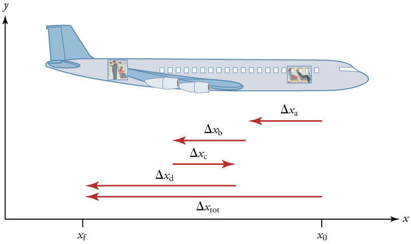
The next several examples consider the motion of the subway train shown in Figure 2.18. In (a) the shuttle moves to the right, and in (b) it moves to the left. The examples are designed to further illustrate aspects of motion and to illustrate some of the reasoning that goes into solving problems.
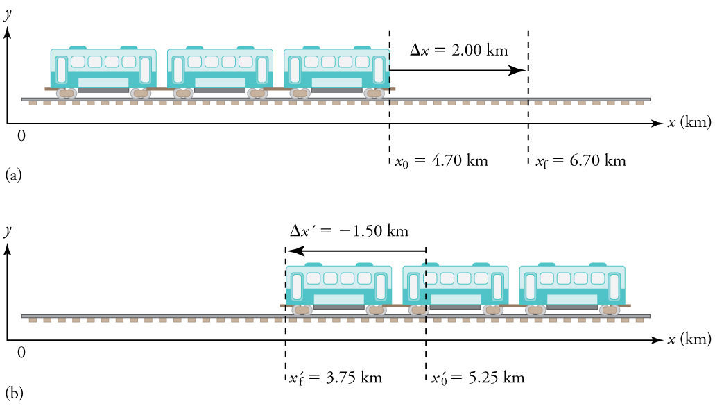
Figure 2.18 One-dimensional motion of a subway train considered in Example 2.2, Example 2.3, Example 2.4, Example 2.5, Example 2.6, and Example 2.7. Here we have chosen the x -axis so that + means to the right and − means to the left for displacements, velocities, and accelerations. (a) The subway train moves to the right from x 0 to x f . Its displacement Δ x is +2.0 km. (b) The train moves to the left from x′0 to x′f . Its displacement Δ x′ is −1.5 km . (Note that the prime symbol (′) is used simply to distinguish between displacement in the two different situations. The distances of travel and the size of the cars are on different scales to fit everything into the diagram.)
Example 2.2 Calculating Displacement: A Subway Train
What are the magnitude and sign of displacements for the motions of the subway train shown in parts (a) and (b) of Figure 2.18?
Strategy
A drawing with a coordinate system is already provided, so we don’t need to make a sketch, but we should analyze it to make sure we
understand what it is showing. Pay particular attention to the coordinate system. To find displacement, we use the equation Δ x = x f − x 0 . This
is straightforward since the initial and final positions are given.
Solution
CHAPTER 2 | KINEMATICS 47
1. Identify the knowns. In the figure we see that x f = 6.70 km and x 0 = 4.70 km for part (a), and x′f = 3.75 km and x′0 = 5.25 km for
part (b).
2. Solve for displacement in part (a).
(2.12)
Δ x = x f − x 0 = 6.70 km − 4.70 km= +2.00 km
3. Solve for displacement in part (b).
(2.13)
Δ x′ = x′f − x′0 = 3.75 km − 5.25 km = − 1.50 km
Discussion
The direction of the motion in (a) is to the right and therefore its displacement has a positive sign, whereas motion in (b) is to the left and thus
has a negative sign.
Example 2.3 Comparing Distance Traveled with Displacement: A Subway Train
What are the distances traveled for the motions shown in parts (a) and (b) of the subway train in Figure 2.18?
Strategy
To answer this question, think about the definitions of distance and distance traveled, and how they are related to displacement. Distance
between two positions is defined to be the magnitude of displacement, which was found in Example 2.2. Distance traveled is the total length of
the path traveled between the two positions. (See Displacement.) In the case of the subway train shown in Figure 2.18, the distance traveled is
the same as the distance between the initial and final positions of the train.
Solution
1. The displacement for part (a) was +2.00 km. Therefore, the distance between the initial and final positions was 2.00 km, and the distance
traveled was 2.00 km.
2. The displacement for part (b) was −1.5 km. Therefore, the distance between the initial and final positions was 1.50 km, and the distance
traveled was 1.50 km.
Discussion
Distance is a scalar. It has magnitude but no sign to indicate direction.
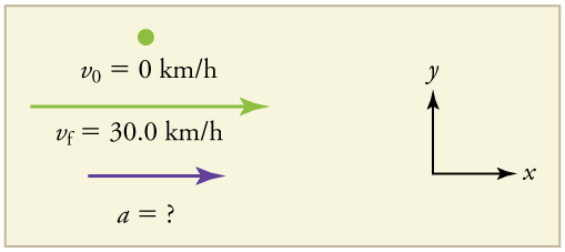
Example 2.4 Calculating Acceleration: A Subway Train Speeding Up
Suppose the train in Figure 2.18(a) accelerates from rest to 30.0 km/h in the first 20.0 s of its motion. What is its average acceleration during that
time interval?
Strategy
It is worth it at this point to make a simple sketch:
Figure 2.19
This problem involves three steps. First we must determine the change in velocity, then we must determine the change in time, and finally we
use these values to calculate the acceleration.
Solution
1. Identify the knowns. v 0 = 0 (the trains starts at rest), v f = 30.0 km/h , and Δ t = 20.0 s .
2. Calculate Δ v . Since the train starts from rest, its change in velocity is Δ v= +30.0 km/h , where the plus sign means velocity to the right.
3. Plug in known values and solve for the unknown, a- .
(2.14)
a- = Δ v