a = Δ v
Δ t
Substituting the simplified notation for Δ v and Δ t gives us
(2.34)
a = v − v 0
t
(constant a).
Solving for v yields
v
(2.35)
= v 0 + at (constant a).
Example 2.9 Calculating Final Velocity: An Airplane Slowing Down after Landing
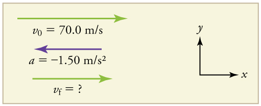
An airplane lands with an initial velocity of 70.0 m/s and then decelerates at 1.50 m/s2 for 40.0 s. What is its final velocity?
Strategy
Draw a sketch. We draw the acceleration vector in the direction opposite the velocity vector because the plane is decelerating.
54 CHAPTER 2 | KINEMATICS
Figure 2.28
Solution
1. Identify the knowns. Δ v = 70.0 m/s , a = −1.50 m/s2 , t = 40.0 s .
2. Identify the unknown. In this case, it is final velocity, v f .
3. Determine which equation to use. We can calculate the final velocity using the equation v = v 0 + at .
4. Plug in the known values and solve.
(2.36)
v = v 0 + at = 70.0 m/s + ⎛⎝−1.50 m/s2⎞⎠(40.0 s) = 10.0 m/s
Discussion
The final velocity is much less than the initial velocity, as desired when slowing down, but still positive. With jet engines, reverse thrust could be
maintained long enough to stop the plane and start moving it backward. That would be indicated by a negative final velocity, which is not the
case here.
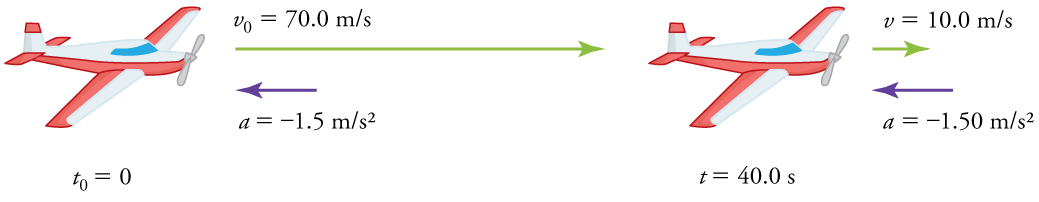
Figure 2.29 The airplane lands with an initial velocity of 70.0 m/s and slows to a final velocity of 10.0 m/s before heading for the terminal. Note that the acceleration is
negative because its direction is opposite to its velocity, which is positive.
In addition to being useful in problem solving, the equation v = v 0 + at gives us insight into the relationships among velocity, acceleration, and
time. From it we can see, for example, that
• final velocity depends on how large the acceleration is and how long it lasts
• if the acceleration is zero, then the final velocity equals the initial velocity ( v = v 0) , as expected (i.e., velocity is constant)
• if a is negative, then the final velocity is less than the initial velocity
(All of these observations fit our intuition, and it is always useful to examine basic equations in light of our intuition and experiences to check that they
do indeed describe nature accurately.)
Making Connections: Real-World Connection
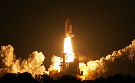
Figure 2.30 The Space Shuttle Endeavor blasts off from the Kennedy Space Center in February 2010. (credit: Matthew Simantov, Flickr)
An intercontinental ballistic missile (ICBM) has a larger average acceleration than the Space Shuttle and achieves a greater velocity in the first
minute or two of flight (actual ICBM burn times are classified—short-burn-time missiles are more difficult for an enemy to destroy). But the Space
CHAPTER 2 | KINEMATICS 55
Shuttle obtains a greater final velocity, so that it can orbit the earth rather than come directly back down as an ICBM does. The Space Shuttle
does this by accelerating for a longer time.
Solving for Final Position When Velocity is Not Constant ( a ≠ 0 )
We can combine the equations above to find a third equation that allows us to calculate the final position of an object experiencing constant
acceleration. We start with
v = v
(2.37)
0 + at.
Adding v 0 to each side of this equation and dividing by 2 gives
v
(2.38)
0 + v
2 = v 0 + 12 at.
v
Since
0 + v
2 = v- for constant acceleration, then
(2.39)
v- = v 0 + 12 at.
Now we substitute this expression for v- into the equation for displacement, x = x 0 + v- t , yielding
(2.40)
x = x 0 + v 0 t + 12 at 2 (constant a).
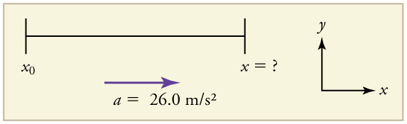
Example 2.10 Calculating Displacement of an Accelerating Object: Dragsters
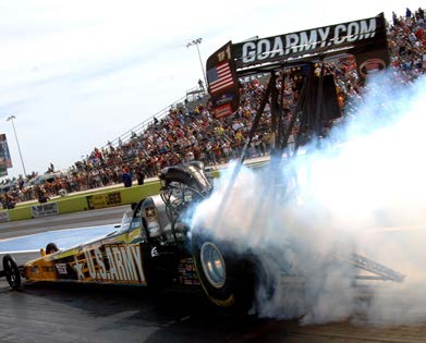
Dragsters can achieve average accelerations of 26.0 m/s2 . Suppose such a dragster accelerates from rest at this rate for 5.56 s. How far does
it travel in this time?
Figure 2.31 U.S. Army Top Fuel pilot Tony “The Sarge” Schumacher begins a race with a controlled burnout. (credit: Lt. Col. William Thurmond. Photo Courtesy of U.S.
Army.)
Strategy
Draw a sketch.
Figure 2.32
We are asked to find displacement, which is x if we take x 0 to be zero. (Think about it like the starting line of a race. It can be anywhere, but
we call it 0 and measure all other positions relative to it.) We can use the equation x = x 0 + v 0 t + 12 at 2 once we identify v 0 , a , and t from the statement of the problem.
Solution
1. Identify the knowns. Starting from rest means that v 0 = 0 , a is given as 26.0 m/s2 and t is given as 5.56 s.

56 CHAPTER 2 | KINEMATICS
2. Plug the known values into the equation to solve for the unknown x :
(2.41)
x = x 0 + v 0 t + 12 at 2.
Since the initial position and velocity are both zero, this simplifies to
(2.42)
x = 12 at 2.
Substituting the identified values of a and t gives
⎛
(2.43)
x = 12⎝26.0 m/s2⎞⎠(5.56 s)2 ,
yielding
x
(2.44)
= 402 m.
Discussion
If we convert 402 m to miles, we find that the distance covered is very close to one quarter of a mile, the standard distance for drag racing. So
the answer is reasonable. This is an impressive displacement in only 5.56 s, but top-notch dragsters can do a quarter mile in even less time than
this.
What else can we learn by examining the equation x = x 0 + v 0 t + 12 at 2? We see that:
• displacement depends on the square of the elapsed time when acceleration is not zero. In Example 2.10, the dragster covers only one fourth of
the total distance in the first half of the elapsed time
• if acceleration is zero, then the initial velocity equals average velocity ( v 0 = v- ) and x = x 0 + v 0 t + 12 at 2 becomes x = x 0 + v 0 t Solving for Final Velocity when Velocity Is Not Constant ( a ≠ 0 )
A fourth useful equation can be obtained from another algebraic manipulation of previous equations.
If we solve v = v 0 + at for t , we get
(2.45)
t = v − v 0
a .
Substituting this and v- = v 0 + v
2
into x = x 0 + v- t , we get
2
(2.46)
v 2 = v 0 + 2 a( x − x 0) (constant a).
Example 2.11 Calculating Final Velocity: Dragsters
Calculate the final velocity of the dragster in Example 2.10 without using information about time.
Strategy
Draw a sketch.
Figure 2.33
The equation v 2 = v 20 + 2 a( x − x 0) is ideally suited to this task because it relates velocities, acceleration, and displacement, and no time information is required.
Solution
1. Identify the known values. We know that v 0 = 0 , since the dragster starts from rest. Then we note that x − x 0 = 402 m (this was the
answer in Example 2.10). Finally, the average acceleration was given to be a = 26.0 m/s2 .
2. Plug the knowns into the equation v 2 = v 20 + 2 a( x − x 0) and solve for v.
CHAPTER 2 | KINEMATICS 57
(2.47)
v 2 = 0 + 2⎛⎝26.0 m/s2⎞⎠(402 m).
Thus
(2.48)
v 2 = 2.09×10⁴ m2 /s2.
To get v , we take the square root:
(2.49)
v = 2.09×10⁴ m2 /s2 = 145 m/s.
Discussion
145 m/s is about 522 km/h or about 324 mi/h, but even this breakneck speed is short of the record for the quarter mile. Also, note that a square
root has two values; we took the positive value to indicate a velocity in the same direction as the acceleration.
An examination of the equation v 2 = v 20 + 2 a( x − x 0) can produce further insights into the general relationships among physical quantities:
• The final velocity depends on how large the acceleration is and the distance over which it acts
• For a fixed deceleration, a car that is going twice as fast doesn’t simply stop in twice the distance—it takes much further to stop. (This is why we
have reduced speed zones near schools.)
Putting Equations Together
In the following examples, we further explore one-dimensional motion, but in situations requiring slightly more algebraic manipulation. The examples
also give insight into problem-solving techniques. The box below provides easy reference to the equations needed.
Summary of Kinematic Equations (constant a )
x
(2.50)
= x 0 + v- t
(2.51)
v- = v 0 + v
2
v = v
(2.52)
0 + at
(2.53)
x = x 0 + v 0 t + 12 at 2
2
(2.54)
v 2 = v 0 + 2 a( x − x 0)
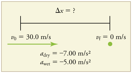
Example 2.12 Calculating Displacement: How Far Does a Car Go When Coming to a Halt?
On dry concrete, a car can decelerate at a rate of 7.00 m/s2 , whereas on wet concrete it can decelerate at only 5.00 m/s2 . Find the distances
necessary to stop a car moving at 30.0 m/s (about 110 km/h) (a) on dry concrete and (b) on wet concrete. (c) Repeat both calculations, finding
the displacement from the point where the driver sees a traffic light turn red, taking into account his reaction time of 0.500 s to get his foot on the
brake.
Strategy
Draw a sketch.
Figure 2.34
In order to determine which equations are best to use, we need to list all of the known values and identify exactly what we need to solve for. We
shall do this explicitly in the next several examples, using tables to set them off.
Solution for (a)
58 CHAPTER 2 | KINEMATICS
1. Identify the knowns and what we want to solve for. We know that v 0 = 30.0 m/s ; v = 0 ; a = −7.00 m/s2 ( a is negative because it is in
a direction opposite to velocity). We take x 0 to be 0. We are looking for displacement Δ x , or x − x 0 .
2. Identify the equation that will help up solve the problem. The best equation to use is
2
(2.55)
v 2 = v 0 + 2 a( x − x 0).
This equation is best because it includes only one unknown, x . We know the values of all the other variables in this equation. (There are other
equations that would allow us to solve for x , but they require us to know the stopping time, t , which we do not know. We could use them but it
would entail additional calculations.)
3. Rearrange the equation to solve for x .
2
(2.56)
v 2
x − x
− v 0
0 =
2 a
4. Enter known values.
(2.57)
x − 0 = 02 − (30.0 m/s)2
2⎛⎝−7.00 m/s2⎞⎠
Thus,
x
(2.58)
= 64.3 m on dry concrete.
Solution for (b)
This part can be solved in exactly the same manner as Part A. The only difference is that the deceleration is – 5.00 m/s2 . The result is
x
(2.59)
wet = 90.0 m on wet concrete.
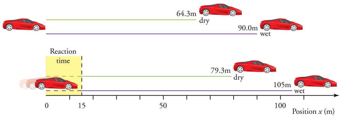
Solution for (c)
Once the driver reacts, the stopping distance is the same as it is in Parts A and B for dry and wet concrete. So to answer this question, we need
to calculate how far the car travels during the reaction time, and then add that to the stopping time. It is reasonable to assume that the velocity
remains constant during the driver’s reaction time.
1. Identify the knowns and what we want to solve for. We know that v- = 30.0 m/s ; t reaction = 0.500 s ; a reaction = 0 . We take x 0 − reaction
to be 0. We are looking for x reaction .
2. Identify the best equation to use.
x = x 0 + v- t works well because the only unknown value is x , which is what we want to solve for.
3. Plug in the knowns to solve the equation.
x
(2.60)
= 0 + (30.0 m/s)(0.500 s) = 15.0 m.
This means the car travels 15.0 m while the driver reacts, making the total displacements in the two cases of dry and wet concrete 15.0 m
greater than if he reacted instantly.
4. Add the displacement during the reaction time to the displacement when braking.
x
(2.61)
braking + x reaction = x total
a. 64.3 m + 15.0 m = 79.3 m when dry
b. 90.0 m + 15.0 m = 105 m when wet
Figure 2.35 The distance necessary to stop a car varies greatly, depending on road conditions and driver reaction time. Shown here are the braking distances for dry and
wet pavement, as calculated in this example, for a car initially traveling at 30.0 m/s. Also shown are the total distances traveled from the point where the driver first sees a
light turn red, assuming a 0.500 s reaction time.
CHAPTER 2 | KINEMATICS 59
Discussion
The displacements found in this example seem reasonable for stopping a fast-moving car. It should take longer to stop a car on wet rather than
dry pavement. It is interesting that reaction time adds significantly to the displacements. But more important is the general approach to solving
problems. We identify the knowns and the quantities to be determined and then find an appropriate equation. There is often more than one way
to solve a problem. The various parts of this example can in fact be solved by other methods, but the solutions presented above are the shortest.
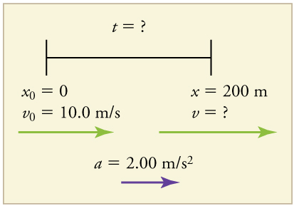
Example 2.13 Calculating Time: A Car Merges into Traffic
Suppose a car merges into freeway traffic on a 200-m-long ramp. If its initial velocity is 10.0 m/s and it accelerates at 2.00 m/s2 , how long does
it take to travel the 200 m up the ramp? (Such information might be useful to a traffic engineer.)
Strategy
Draw a sketch.
Figure 2.36
We are asked to solve for the time t . As before, we identify the known quantities in order to choose a convenient physical relationship (that is,
an equation with one unknown, t ).
Solution
1. Identify the knowns and what we want to solve for. We know that v 0 = 10 m/s ; a = 2.00 m/s2 ; and x = 200 m .
2. We need to solve for t . Choose the best equation. x = x 0 + v 0 t + 12 at 2 works best because the only unknown in the equation is the variable t for which we need to solve.
3. We will need to rearrange the equation to solve for t . In this case, it will be easier to plug in the knowns first.
⎛
(2.62)
200 m = 0 m + (10.0 m/s) t + 12⎝2.00 m/s2⎞⎠ t 2
4. Simplify the equation. The units of meters (m) cancel because they are in each term. We can get the units of seconds (s) to cancel by taking
t = t s , where t is the magnitude of time and s is the unit. Doing so leaves
(2.63)
200 = 10 t + t 2.
5. Use the quadratic formula to solve for t .
(a) Rearrange the equation to get 0 on one side of the equation.
(2.64)
t 2 + 10 t − 200 = 0
This is a quadratic equation of the form
(2.65)
at 2 + bt + c = 0,
where the constants are a = 1.00, b = 10.0, and c = −200 .
(b) Its solutions are given by the quadratic formula:
(2.66)
t = − b ± b 2 − 4 ac
2 a
.
This yields two solutions for t , which are
t
(2.67)
= 10.0 and−20.0.
In this case, then, the time is t = t in seconds, or
t
(2.68)
= 10.0 s and − 20.0 s.
60 CHAPTER 2 | KINEMATICS
A negative value for time is unreasonable, since it would mean that the event happened 20 s before the motion began. We can discard that
solution. Thus,
t
(2.69)
= 10.0 s.
Discussion
Whenever an equation contains an unknown squared, there will be two solutions. In some problems both solutions are meaningful, but in others,
such as the above, only one solution is reasonable. The 10.0 s answer seems reasonable for a typical freeway on-ramp.
With the basics of kinematics established, we can go on to many other interesting examples and applications. In the process of developing
kinematics, we have also glimpsed a general approach to problem solving that produces both correct answers and insights into physical
relationships. Problem-Solving Basics discusses problem-solving basics and outlines an approach that will help you succeed in this invaluable task.
Making Connections: Take-Home Experiment—Breaking News
We have been using SI units of meters per second squared to describe some examples of acceleration or deceleration of cars, runners, and
trains. To achieve a better feel for these numbers, one can measure the braking deceleration of a car doing a slow (and safe) stop. Recall that,
for average acceleration, a- = Δ v / Δ t . While traveling in a car, slowly apply the brakes as you come up to a stop sign. Have a passenger note
the initial speed in miles per hour and the time taken (in seconds) to stop. From this, calculate the deceleration in miles per hour per second.
Convert this to meters per second squared and compare with other decelerations mentioned in this chapter. Calculate the distance traveled in
braking.
A manned rocket accelerates at a rate of 20 m/s2 during launch. How long does it take the rocket reach a velocity of 400 m/s?
Solution
To answer this, choose an equation that allows you to solve for time t , given only a , v 0 , and v .
v = v
(2.70)
0 + at
Rearrange to solve for t .
(2.71)
t = v − v
a = 400 m/s − 0 m/s
20 m/s2
= 20 s
2.6 Problem-Solving Basics for One-Dimensional Kinematics
Figure 2.37 Problem-solving skills are essential to your success in Physics. (credit: scui3asteveo, Flickr)
Problem-solving skills are obviously essential to success in a quantitative course in physics. More importantly, the ability to apply broad physical
principles, usually represented by equations, to specific situations is a very powerful form of knowledge. It is much more powerful than memorizing a
list of facts. Analytical skills and problem-solving abilities can be applied to new situations, whereas a list of facts cannot be made long enough to
contain every possible circumstance. Such analytical skills are useful both for solving problems in this text and for applying physics in everyday and
professional life.
Problem-Solving Steps