and find out if it is positive or negative.
Solution for Velocity v 1
1. Identify the knowns. We know that y 0 = 0 ; v 0 = 13.0 m/s ; a = − g = −9.80 m/s2 ; and t = 1.00 s . We also know from the solution
above that y 1 = 8.10 m .
2. Identify the best equation to use. The most straightforward is v = v 0 − gt (from v = v 0 + at , where
a = gravitational acceleration = − g ).
3. Plug in the knowns and solve.
(2.79)
v 1 = v 0 − gt = 13.0 m/s − ⎛⎝9.80 m/s2⎞⎠(1.00 s) = 3.20 m/s
Discussion
The positive value for v 1 means that the rock is still heading upward at t = 1.00 s . However, it has slowed from its original 13.0 m/s, as
expected.
Solution for Remaining Times
The procedures for calculating the position and velocity at t = 2.00 s and 3.00 s are the same as those above. The results are summarized in
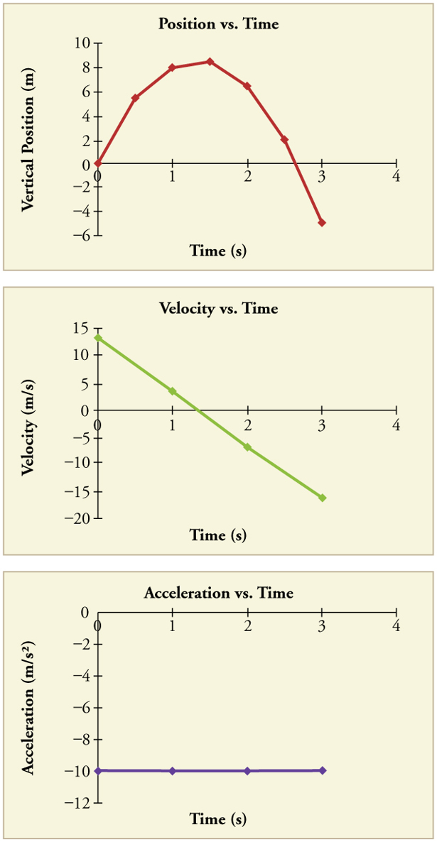
Table 2.1 and illustrated in Figure 2.40.
Table 2.1 Results
Time, t
Position, y
Velocity, v
Acceleration, a
1.00 s
8.10 m
3.20 m/s
−9.80 m/s2
2.00 s
6.40 m
−6.60 m/s
−9.80 m/s2
3.00 s
−5.10 m
−16.4 m/s
−9.80 m/s2
Graphing the data helps us understand it more clearly.
64 CHAPTER 2 | KINEMATICS
Figure 2.40 Vertical position, vertical velocity, and vertical acceleration vs. time for a rock thrown vertically up at the edge of a cliff. Notice that velocity changes linearly with time and that acceleration is constant. Misconception Alert! Notice that the position vs. time graph shows vertical position only. It is easy to get the impression that
the graph shows some horizontal motion—the shape of the graph looks like the path of a projectile. But this is not the case; the horizontal axis is time, not space. The
actual path of the rock in space is straight up, and straight down.
Discussion
The interpretation of these results is important. At 1.00 s the rock is above its starting point and heading upward, since y 1 and v 1 are both
positive. At 2.00 s, the rock is still above its starting point, but the negative velocity means it is moving downward. At 3.00 s, both y 3 and v 3
are negative, meaning the rock is below its starting point and continuing to move downward. Notice that when the rock is at its highest point (at
1.5 s), its velocity is zero, but its acceleration is still −9.80 m/s2 . Its acceleration is −9.80 m/s2 for the whole trip—while it is moving up and
while it is moving down. Note that the values for y are the positions (or displacements) of the rock, not the total distances traveled. Finally, note
that free-fall applies to upward motion as well as downward. Both have the same acceleration—the acceleration due to gravity, which remains
constant the entire time. Astronauts training in the famous Vomit Comet, for example, experience free-fall while arcing up as well as down, as we
will discuss in more detail later.
Making Connections: Take-Home Experiment—Reaction Time
A simple experiment can be done to determine your reaction time. Have a friend hold a ruler between your thumb and index finger, separated by
about 1 cm. Note the mark on the ruler that is right between your fingers. Have your friend drop the ruler unexpectedly, and try to catch it
between your two fingers. Note the new reading on the ruler. Assuming acceleration is that due to gravity, calculate your reaction time. How far
would you travel in a car (moving at 30 m/s) if the time it took your foot to go from the gas pedal to the brake was twice this reaction time?
CHAPTER 2 | KINEMATICS 65
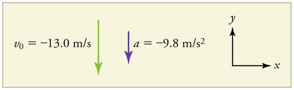
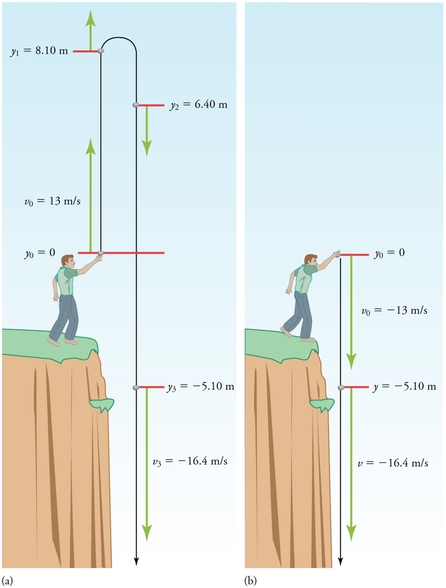
Example 2.15 Calculating Velocity of a Falling Object: A Rock Thrown Down
What happens if the person on the cliff throws the rock straight down, instead of straight up? To explore this question, calculate the velocity of the
rock when it is 5.10 m below the starting point, and has been thrown downward with an initial speed of 13.0 m/s.
Strategy
Draw a sketch.
Figure 2.41
Since up is positive, the final position of the rock will be negative because it finishes below the starting point at y 0 = 0 . Similarly, the initial
velocity is downward and therefore negative, as is the acceleration due to gravity. We expect the final velocity to be negative since the rock will
continue to move downward.
Solution
1. Identify the knowns. y 0 = 0 ; y 1 = − 5.10 m ; v 0 = −13.0 m/s ; a = − g = −9.80 m/s2 .
2. Choose the kinematic equation that makes it easiest to solve the problem. The equation v 2 = v 20 + 2 a( y − y 0) works well because the only
unknown in it is v . (We will plug y 1 in for y .)
3. Enter the known values
(2.80)
v 2 = (−13.0 m/s)2 + 2⎛⎝−9.80 m/s2⎞⎠(−5.10 m − 0 m) = 268.96 m2 /s2,
where we have retained extra significant figures because this is an intermediate result.
Taking the square root, and noting that a square root can be positive or negative, gives
v
(2.81)
= ±16.4 m/s.
The negative root is chosen to indicate that the rock is still heading down. Thus,
v
(2.82)
= −16.4 m/s.
Discussion
Note that this is exactly the same velocity the rock had at this position when it was thrown straight upward with the same initial speed. (See
Example 2.14 and Figure 2.42(a).) This is not a coincidental result. Because we only consider the acceleration due to gravity in this problem, the speed of a falling object depends only on its initial speed and its vertical position relative to the starting point. For example, if the velocity of
the rock is calculated at a height of 8.10 m above the starting point (using the method from Example 2.14) when the initial velocity is 13.0 m/s
straight up, a result of ±3.20 m/s is obtained. Here both signs are meaningful; the positive value occurs when the rock is at 8.10 m and
heading up, and the negative value occurs when the rock is at 8.10 m and heading back down. It has the same speed but the opposite direction.
66 CHAPTER 2 | KINEMATICS
Figure 2.42 (a) A person throws a rock straight up, as explored in Example 2.14. The arrows are velocity vectors at 0, 1.00, 2.00, and 3.00 s. (b) A person throws a rock
straight down from a cliff with the same initial speed as before, as in Example 2.15. Note that at the same distance below the point of release, the rock has the same
velocity in both cases.
Another way to look at it is this: In Example 2.14, the rock is thrown up with an initial velocity of 13.0 m/s . It rises and then falls back down.
When its position is y = 0 on its way back down, its velocity is −13.0 m/s . That is, it has the same speed on its way down as on its way up.
We would then expect its velocity at a position of y = −5.10 m to be the same whether we have thrown it upwards at +13.0 m/s or thrown it
downwards at −13.0 m/s . The velocity of the rock on its way down from y = 0 is the same whether we have thrown it up or down to start
with, as long as the speed with which it was initially thrown is the same.
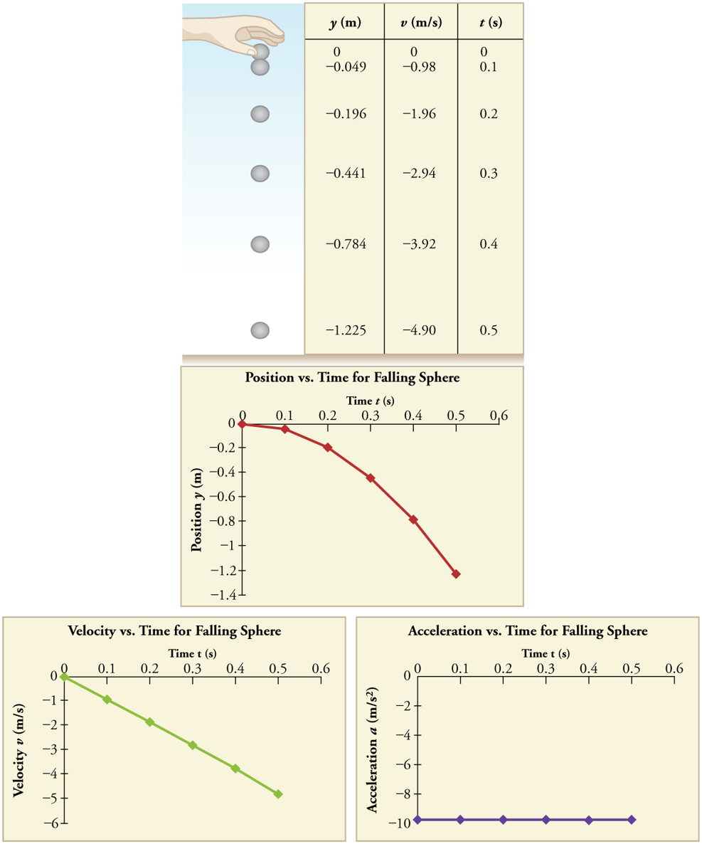
Example 2.16 Find g from Data on a Falling Object
The acceleration due to gravity on Earth differs slightly from place to place, depending on topography (e.g., whether you are on a hill or in a
valley) and subsurface geology (whether there is dense rock like iron ore as opposed to light rock like salt beneath you.) The precise
acceleration due to gravity can be calculated from data taken in an introductory physics laboratory course. An object, usually a metal ball for
which air resistance is negligible, is dropped and the time it takes to fall a known distance is measured. See, for example, Figure 2.43. Very
precise results can be produced with this method if sufficient care is taken in measuring the distance fallen and the elapsed time.
CHAPTER 2 | KINEMATICS 67
Figure 2.43 Positions and velocities of a metal ball released from rest when air resistance is negligible. Velocity is seen to increase linearly with time while displacement
increases with time squared. Acceleration is a constant and is equal to gravitational acceleration.
Suppose the ball falls 1.0000 m in 0.45173 s. Assuming the ball is not affected by air resistance, what is the precise acceleration due to gravity at
this location?
Strategy
Draw a sketch.
Figure 2.44
We need to solve for acceleration a . Note that in this case, displacement is downward and therefore negative, as is acceleration.
Solution

68 CHAPTER 2 | KINEMATICS
1. Identify the knowns. y 0 = 0 ; y = –1.0000 m ; t = 0.45173 ; v 0 = 0 .
2. Choose the equation that allows you to solve for a using the known values.
(2.83)
y = y 0 + v 0 t + 12 at 2
3. Substitute 0 for v 0 and rearrange the equation to solve for a . Substituting 0 for v 0 yields
(2.84)
y = y 0 + 12 at 2.
Solving for a gives
(2.85)
a = 2( y − y 0)
t 2
.
4. Substitute known values yields
(2.86)
a = 2( − 1.0000 m – 0)
(0.45173 s)2
= −9.8010 m/s2 ,
so, because a = − g with the directions we have chosen,
(2.87)
g = 9.8010 m/s2.
Discussion
The negative value for a indicates that the gravitational acceleration is downward, as expected. We expect the value to be somewhere around
the average value of 9.80 m/s2 , so 9.8010 m/s2 makes sense. Since the data going into the calculation are relatively precise, this value for
g is more precise than the average value of 9.80 m/s2 ; it represents the local value for the acceleration due to gravity.
A chunk of ice breaks off a glacier and falls 30.0 meters before it hits the water. Assuming it falls freely (there is no air resistance), how long does
it take to hit the water?
Solution
We know that initial position y 0 = 0 , final position y = −30.0 m , and a = − g = −9.80 m/s2 . We can then use the equation
y = y 0 + v 0 t + 12 at 2 to solve for t . Inserting a = − g, we obtain
(2.88)
y = 0 + 0 − 12 gt 2
t 2 = 2 y
− g
t = ± 2 y
− g = ± 2( − 30.0 m)
−9.80 m/s2 = ± 6.12 s2 = 2.47 s ≈ 2.5 s
where we take the positive value as the physically relevant answer. Thus, it takes about 2.5 seconds for the piece of ice to hit the water.
PhET Explorations: Equation Grapher
Learn about graphing polynomials. The shape of the curve changes as the constants are adjusted. View the curves for the individual terms (e.g.
y = bx ) to see how they add to generate the polynomial curve.
Figure 2.45 Equation Grapher (http://cnx.org/content/m42102/1.3/equation-grapher_en.jar)
2.8 Graphical Analysis of One-Dimensional Motion
A graph, like a picture, is worth a thousand words. Graphs not only contain numerical information; they also reveal relationships between physical
quantities. This section uses graphs of displacement, velocity, and acceleration versus time to illustrate one-dimensional kinematics.
CHAPTER 2 | KINEMATICS 69
Slopes and General Relationships
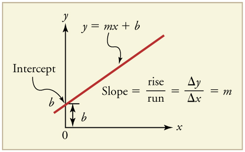
First note that graphs in this text have perpendicular axes, one horizontal and the other vertical. When two physical quantities are plotted against one
another in such a graph, the horizontal axis is usually considered to be an independent variable and the vertical axis a dependent variable. If we
call the horizontal axis the x -axis and the vertical axis the y -axis, as in Figure 2.46, a straight-line graph has the general form
y
(2.89)
= mx + b.
Here m is the slope, defined to be the rise divided by the run (as seen in the figure) of the straight line. The letter b is used for the y-intercept, which is the point at which the line crosses the vertical axis.
Figure 2.46 A straight-line graph. The equation for a straight line is y = mx + b .
Graph of Displacement vs. Time ( a = 0, so v is constant)
Time is usually an independent variable that other quantities, such as displacement, depend upon. A graph of displacement versus time would, thus,
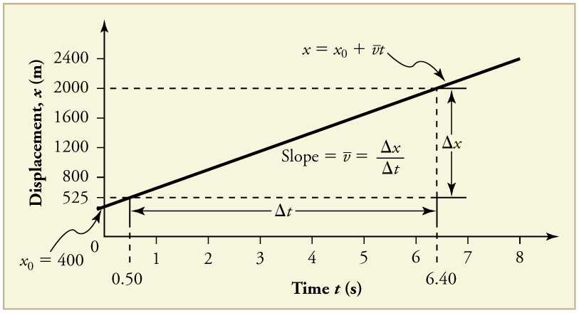
have x on the vertical axis and t on the horizontal axis. Figure 2.47 is just such a straight-line graph. It shows a graph of displacement versus time for a jet-powered car on a very flat dry lake bed in Nevada.
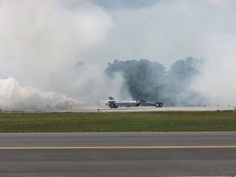
Figure 2.47 Graph of displacement versus time for a jet-powered car on the Bonneville Salt Flats.
Using the relationship between dependent and independent variables, we see that the slope in the graph above is average velocity v- and the
intercept is displacement at time zero—that is, x 0 . Substituting these symbols into y = mx + b gives
x
(2.90)
= v- t + x 0
or
x
(2.91)
= x 0 + v- t.
Thus a graph of displacement versus time gives a general relationship among displacement, velocity, and time, as well as giving detailed numerical
information about a specific situation.
The Slope of x vs. t
The slope of the graph of displacement x vs. time t is velocity v .
(2.92)
slope = Δ x
Δ t = v
70 CHAPTER 2 | KINEMATICS
Notice that this equation is the same as that derived algebraically from other motion equations in Motion Equations for Constant Acceleration
From the figure we can see that the car has a displacement of 400 m at time 0.650 m at t = 1.0 s, and so on. Its displacement at times other than
those listed in the table can be read from the graph; furthermore, information about its velocity and acceleration can also be obtained from the graph.
Example 2.17 Determining Average Velocity from a Graph of Displacement versus Time: Jet Car
Find the average velocity of the car whose position is graphed in Figure 2.47.
Strategy
The slope of a graph of x vs. t is average velocity, since slope equals rise over run. In this case, rise = change in displacement and run =
change in time, so that
(2.93)
slope = Δ x
Δ t = v- .
Since the slope is constant here, any two points on the graph can be used to find the slope. (Generally speaking, it is most accurate to use two
widely separated points on the straight line. This is because any error in reading data from the graph is proportionally smaller if the interval is
larger.)
Solution
1. Choose two points on the line. In this case, we choose the points labeled on the graph: (6.4 s, 2000 m) and (0.50 s, 525 m). (Note, however,
that you could choose any two points.)
2. Substitute the x and t values of the chosen points into the equation. Remember in calculating change (Δ) we always use final value minus
initial value.
(2.94)
v- = Δ x
Δ t = 2000 m − 525 m
6.4 s − 0.50 s ,
yielding
v-
(2.95)
= 250 m/s.
Discussion
This is an impressively large land speed (900 km/h, or about 560 mi/h): much greater than the typical highway speed limit of 60 mi/h (27 m/s or
96 km/h), but considerably shy of the record of 343 m/s (1234 km/h or 766 mi/h) set in 1997.
Graphs of Motion when a is constant but a ≠ 0
The graphs in Figure 2.48 below represent the motion of the jet-powered car as it accelerates toward its top speed, but only during the time when its acceleration is constant. Time starts at zero for this motion (as if measured with a stopwatch), and the displacement and velocity are initially 200 m
and 15 m/s, respectively.
CHAPTER 2 | KINEMATICS 71
Figure 2.48 Graphs of motion of a jet-powered car during the time span when its acceleration is constant. (a) The slope of an x vs. t graph is velocity. This is shown at two points, and the instantaneous velocities obtained are plotted in the next graph. Instantaneous velocity at any point is the slope of the tangent at that point. (b) The slope of the
v vs. t graph is constant for this part of the motion, indicating constant acceleration. (c) Acceleration has the constant value of 5.0 m/s2 over the time interval plotted.
72 CHAPTER 2 | KINEMATICS
Figure 2.49 A U.S. Air Force jet car speeds down a track. (credit: Matt Trostle, Flickr)
The graph of displacement versus time in Figure 2.48(a) is a curve rather than a straight line. The slope of the curve becomes steeper as time
progresses, showing that the velocity is increasing over time. The slope at any point on a displacement-versus-time graph is the instantaneous
velocity at that point. It is found by drawing a straight line tangent to the curve at the point of interest and taking the slope of this straight line. Tangent
lines are shown for two points in Figure 2.48(a). If this is done at every point on the curve and the values are plotted against time, then the graph of
velocity versus time shown in Figure 2.48(b) is obtained. Furthermore, the slope of the graph of velocity versus time is acceleration, which is shown in Figure 2.48(c).
Example 2.18 Determining Instantaneous Velocity from the Slope at a Point: Jet Car
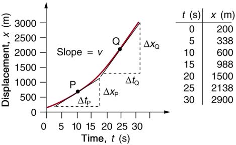
Calculate the velocity of the jet car at a time of 25 s by finding the slope of the x vs. t graph in the graph below.
Figure 2.50 The slope of an x vs. t graph is velocity. This is shown at two points. Instantaneous velocity at any point is the slope of the tangent at that point.
Strategy
The slope of a curve at a point is equal to the slope of a straight line tangent to the curve at that point. This principle is illustrated in Figure 2.50, where Q is the point at t = 25 s .
Solution
1. Find the tangent line to the curve at t = 25 s .
2. Determine the endpoints of the tangent. These correspond to a position of 1300 m at time 19 s and a position of 3120 m at time 32 s.
3. Plug these endpoints into the equation to solve for the slope, v .
(2.96)
Δ x
slope = v
Q
Q = Δ t = (3120 m − 1300 m)
Q
(32 s − 19 s)
Thus,
(2.97)
v Q = 1820 m
13 s = 140 m/s.
Discussion
This is the value given in this figure’s table for v at t = 25 s . The value of 140 m/s for v Q is plotted in Figure 2.50. The entire graph of v vs.
t can be obtained in this fashion.
Carrying this one step further, we note that the slope of a velocity versus time graph is acceleration. Slope is rise divided by run; on a v vs. t graph,
rise = change in velocity Δ v and run = change in time Δ t .
CHAPTER 2 | KINEMATICS 73
The Slope of v vs. t
The slope of a graph of velocity v vs. time t is acceleration a .
(2.98)
slope = Δ v
Δ t = a
Since the velocity versus time graph in Figure 2.48(b) is a straight line, its slope is the same everywhere, implying that acceleration is constant.
Acceleration versus time is graphed in Figu