86 CHAPTER 3 | TWO-DIMENSIONAL KINEMATICS
Introduction to Two-Dimensional Kinematics
The arc of a basketball, the orbit of a satellite, a bicycle rounding a curve, a swimmer diving into a pool, blood gushing out of a wound, and a puppy
chasing its tail are but a few examples of motions along curved paths. In fact, most motions in nature follow curved paths rather than straight lines.
Motion along a curved path on a flat surface or a plane (such as that of a ball on a pool table or a skater on an ice rink) is two-dimensional, and thus
described by two-dimensional kinematics. Motion not confined to a plane, such as a car following a winding mountain road, is described by three-
dimensional kinematics. Both two- and three-dimensional kinematics are simple extensions of the one-dimensional kinematics developed for straight-
line motion in the previous chapter. This simple extension will allow us to apply physics to many more situations, and it will also yield unexpected
insights about nature.
3.1 Kinematics in Two Dimensions: An Introduction
Figure 3.2 Walkers and drivers in a city like New York are rarely able to travel in straight lines to reach their destinations. Instead, they must follow roads and sidewalks,
making two-dimensional, zigzagged paths. (credit: Margaret W. Carruthers)
Two-Dimensional Motion: Walking in a City
Suppose you want to walk from one point to another in a city with uniform square blocks, as pictured in Figure 3.3.
Figure 3.3 A pedestrian walks a two-dimensional path between two points in a city. In this scene, all blocks are square and are the same size.
The straight-line path that a helicopter might fly is blocked to you as a pedestrian, and so you are forced to take a two-dimensional path, such as the
one shown. You walk 14 blocks in all, 9 east followed by 5 north. What is the straight-line distance?
An old adage states that the shortest distance between two points is a straight line. The two legs of the trip and the straight-line path form a right
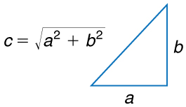
triangle, and so the Pythagorean theorem, a 2 + b 2 = c 2 , can be used to find the straight-line distance.
Figure 3.4 The Pythagorean theorem relates the length of the legs of a right triangle, labeled a and b , with the hypotenuse, labeled c . The relationship is given by: a 2 + b 2 = c 2 . This can be rewritten, solving for c : c = a 2 + b 2 .
The hypotenuse of the triangle is the straight-line path, and so in this case its length in units of city blocks is
(9 blocks)2+ (5 blocks)2= 10.3 blocks , considerably shorter than the 14 blocks you walked. (Note that we are using three significant figures in
CHAPTER 3 | TWO-DIMENSIONAL KINEMATICS 87
the answer. Although it appears that “9” and “5” have only one significant digit, they are discrete numbers. In this case “9 blocks” is the same as “9.0
or 9.00 blocks.” We have decided to use three significant figures in the answer in order to show the result more precisely.)
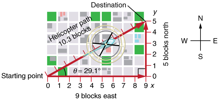
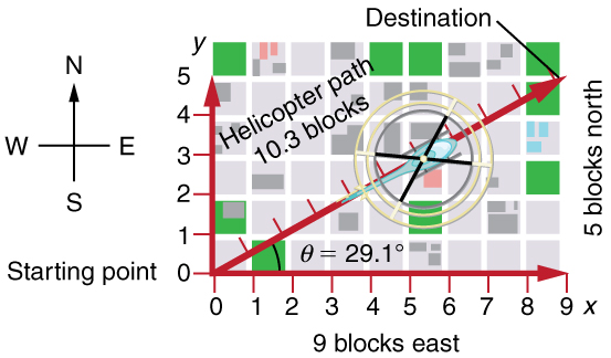
Figure 3.5 The straight-line path followed by a helicopter between the two points is shorter than the 14 blocks walked by the pedestrian. All blocks are square and the same
size.
The fact that the straight-line distance (10.3 blocks) in Figure 3.5 is less than the total distance walked (14 blocks) is one example of a general
characteristic of vectors. (Recall that vectors are quantities that have both magnitude and direction.)
As for one-dimensional kinematics, we use arrows to represent vectors. The length of the arrow is proportional to the vector’s magnitude. The arrow’s
length is indicated by hash marks in Figure 3.3 and Figure 3.5. The arrow points in the same direction as the vector. For two-dimensional motion, the path of an object can be represented with three vectors: one vector shows the straight-line path between the initial and final points of the motion, one
vector shows the horizontal component of the motion, and one vector shows the vertical component of the motion. The horizontal and vertical
components of the motion add together to give the straight-line path. For example, observe the three vectors in Figure 3.5. The first represents a
9-block displacement east. The second represents a 5-block displacement north. These vectors are added to give the third vector, with a 10.3-block
total displacement. The third vector is the straight-line path between the two points. Note that in this example, the vectors that we are adding are
perpendicular to each other and thus form a right triangle. This means that we can use the Pythagorean theorem to calculate the magnitude of the
total displacement. (Note that we cannot use the Pythagorean theorem to add vectors that are not perpendicular. We will develop techniques for
adding vectors having any direction, not just those perpendicular to one another, in Vector Addition and Subtraction: Graphical Methods and
Vector Addition and Subtraction: Analytical Methods.)
The Independence of Perpendicular Motions
The person taking the path shown in Figure 3.5 walks east and then north (two perpendicular directions). How far he or she walks east is only
affected by his or her motion eastward. Similarly, how far he or she walks north is only affected by his or her motion northward.
Independence of Motion
The horizontal and vertical components of two-dimensional motion are independent of each other. Any motion in the horizontal direction does not
affect motion in the vertical direction, and vice versa.
This is true in a simple scenario like that of walking in one direction first, followed by another. It is also true of more complicated motion involving
movement in two directions at once. For example, let’s compare the motions of two baseballs. One baseball is dropped from rest. At the same
instant, another is thrown horizontally from the same height and follows a curved path. A stroboscope has captured the positions of the balls at fixed
time intervals as they fall.
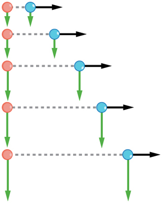
Figure 3.6 This shows the motions of two identical balls—one falls from rest, the other has an initial horizontal velocity. Each subsequent position is an equal time interval.
Arrows represent horizontal and vertical velocities at each position. The ball on the right has an initial horizontal velocity, while the ball on the left has no horizontal velocity.
Despite the difference in horizontal velocities, the vertical velocities and positions are identical for both balls. This shows that the vertical and horizontal motions are
independent.
It is remarkable that for each flash of the strobe, the vertical positions of the two balls are the same. This similarity implies that the vertical motion is
independent of whether or not the ball is moving horizontally. (Assuming no air resistance, the vertical motion of a falling object is influenced by
gravity only, and not by any horizontal forces.) Careful examination of the ball thrown horizontally shows that it travels the same horizontal distance
between flashes. This is due to the fact that there are no additional forces on the ball in the horizontal direction after it is thrown. This result means

88 CHAPTER 3 | TWO-DIMENSIONAL KINEMATICS
that the horizontal velocity is constant, and affected neither by vertical motion nor by gravity (which is vertical). Note that this case is true only for ideal
conditions. In the real world, air resistance will affect the speed of the balls in both directions.
The two-dimensional curved path of the horizontally thrown ball is composed of two independent one-dimensional motions (horizontal and vertical).
The key to analyzing such motion, called projectile motion, is to resolve (break) it into motions along perpendicular directions. Resolving two-
dimensional motion into perpendicular components is possible because the components are independent. We shall see how to resolve vectors in
Vector Addition and Subtraction: Graphical Methods and Vector Addition and Subtraction: Analytical Methods. We will find such techniques to be useful in many areas of physics.
PhET Explorations: Ladybug Motion 2D
Learn about position, velocity and acceleration vectors. Move the ladybug by setting the position, velocity or acceleration, and see how the
vectors change. Choose linear, circular or elliptical motion, and record and playback the motion to analyze the behavior.
Figure 3.7 Ladybug Motion 2D (http://cnx.org/content/m42104/1.4/ladybug-motion-2d_en.jar)
3.2 Vector Addition and Subtraction: Graphical Methods
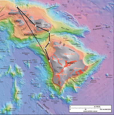
Figure 3.8 Displacement can be determined graphically using a scale map, such as this one of the Hawaiian Islands. A journey from Hawai’i to Moloka’i has a number of legs,
or journey segments. These segments can be added graphically with a ruler to determine the total two-dimensional displacement of the journey. (credit: US Geological Survey)
Vectors in Two Dimensions
A vector is a quantity that has magnitude and direction. Displacement, velocity, acceleration, and force, for example, are all vectors. In one-
dimensional, or straight-line, motion, the direction of a vector can be given simply by a plus or minus sign. In two dimensions (2-d), however, we
specify the direction of a vector relative to some reference frame (i.e., coordinate system), using an arrow having length proportional to the vector’s
magnitude and pointing in the direction of the vector.
Figure 3.9 shows such a graphical representation of a vector, using as an example the total displacement for the person walking in a city considered in Kinematics in Two Dimensions: An Introduction. We shall use the notation that a boldface symbol, such as D , stands for a vector. Its
magnitude is represented by the symbol in italics, D , and its direction by θ .
Vectors in this Text
In this text, we will represent a vector with a boldface variable. For example, we will represent the quantity force with the vector F , which has
both magnitude and direction. The magnitude of the vector will be represented by a variable in italics, such as F , and the direction of the
variable will be given by an angle θ .
CHAPTER 3 | TWO-DIMENSIONAL KINEMATICS 89
Figure 3.9 A person walks 9 blocks east and 5 blocks north. The displacement is 10.3 blocks at an angle 29.1º north of east.
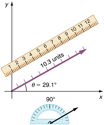
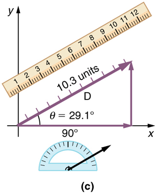
Figure 3.10 To describe the resultant vector for the person walking in a city considered in Figure 3.9 graphically, draw an arrow to represent the total displacement vector D .
Using a protractor, draw a line at an angle θ relative to the east-west axis. The length D of the arrow is proportional to the vector’s magnitude and is measured along the line with a ruler. In this example, the magnitude D of the vector is 10.3 units, and the direction θ is 29.1º north of east.
Vector Addition: Head-to-Tail Method
The head-to-tail method is a graphical way to add vectors, described in Figure 3.11 below and in the steps following. The tail of the vector is the starting point of the vector, and the head (or tip) of a vector is the final, pointed end of the arrow.
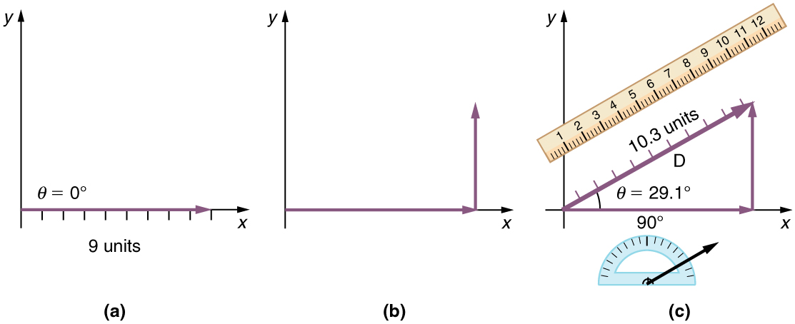
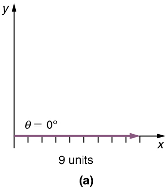
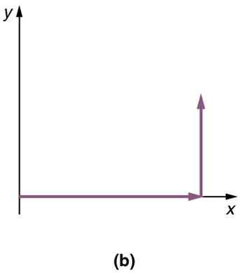
Figure 3.11 Head-to-Tail Method: The head-to-tail method of graphically adding vectors is illustrated for the two displacements of the person walking in a city considered in
Figure 3.9. (a) Draw a vector representing the displacement to the east. (b) Draw a vector representing the displacement to the north. The tail of this vector should originate from the head of the first, east-pointing vector. (c) Draw a line from the tail of the east-pointing vector to the head of the north-pointing vector to form the sum or resultant
vector D . The length of the arrow D is proportional to the vector’s magnitude and is measured to be 10.3 units . Its direction, described as the angle with respect to the east (or horizontal axis) θ is measured with a protractor to be 29.1º .
Step 1. Draw an arrow to represent the first vector (9 blocks to the east) using a ruler and protractor.
90 CHAPTER 3 | TWO-DIMENSIONAL KINEMATICS
Figure 3.12
Step 2. Now draw an arrow to represent the second vector (5 blocks to the north). Place the tail of the second vector at the head of the first vector.
Figure 3.13
Step 3. If there are more than two vectors, continue this process for each vector to be added. Note that in our example, we have only two vectors, so
we have finished placing arrows tip to tail.
Step 4. Draw an arrow from the tail of the first vector to the head of the last vector. This is the resultant, or the sum, of the other vectors.
Figure 3.14
Step 5. To get the magnitude of the resultant, measure its length with a ruler. (Note that in most calculations, we will use the Pythagorean theorem to
determine this length.)
Step 6. To get the direction of the resultant, measure the angle it makes with the reference frame using a protractor. (Note that in most calculations,
we will use trigonometric relationships to determine this angle.)
The graphical addition of vectors is limited in accuracy only by the precision with which the drawings can be made and the precision of the measuring
tools. It is valid for any number of vectors.
CHAPTER 3 | TWO-DIMENSIONAL KINEMATICS 91
Example 3.1 Adding Vectors Graphically Using the Head-to-Tail Method: A Woman Takes a Walk
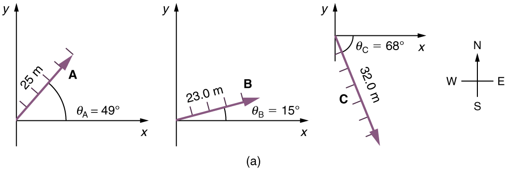
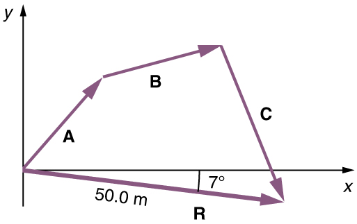
Use the graphical technique for adding vectors to find the total displacement of a person who walks the following three paths (displacements) on
a flat field. First, she walks 25.0 m in a direction 49.0º north of east. Then, she walks 23.0 m heading 15.0º north of east. Finally, she turns
and walks 32.0 m in a direction 68.0° south of east.
Strategy
Represent each displacement vector graphically with an arrow, labeling the first A , the second B , and the third C , making the lengths
proportional to the distance and the directions as specified relative to an east-west line. The head-to-tail method outlined above will give a way to
determine the magnitude and direction of the resultant displacement, denoted R .
Solution
(1) Draw the three displacement vectors.
Figure 3.15
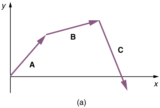
(2) Place the vectors head to tail retaining both their initial magnitude and direction.
Figure 3.16
(3) Draw the resultant vector, R .
Figure 3.17
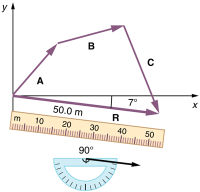
(4) Use a ruler to measure the magnitude of R , and a protractor to measure the direction of R . While the direction of the vector can be
specified in many ways, the easiest way is to measure the angle between the vector and the nearest horizontal or vertical axis. Since the
resultant vector is south of the eastward pointing axis, we flip the protractor upside down and measure the angle between the eastward axis and
the vector.
92 CHAPTER 3 | TWO-DIMENSIONAL KINEMATICS
Figure 3.18
In this case, the total displacement R is seen to have a magnitude of 50.0 m and to lie in a direction 7.0º south of east. By using its magnitude
and direction, this vector can be expressed as R = 50.0 m and θ = 7.0º south of east.
Discussion
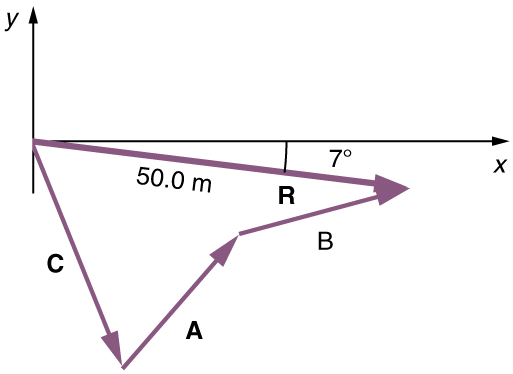
The head-to-tail graphical method of vector addition works for any number of vectors. It is also important to note that the resultant is independent
of the order in which the vectors are added. Therefore, we could add the vectors in any order as illustrated in Figure 3.19 and we will still get the same solution.
Figure 3.19
Here, we see that when the same vectors are added in a different order, the result is the same. This characteristic is true in every case and is an
important characteristic of vectors. Vector addition is commutative. Vectors can be added in any order.
(3.1)
A + B = B + A.
(This is true for the addition of ordinary numbers as well—you get the same result whether you add 2 + 3 or 3 + 2 , for example).
Vector Subtraction
Vector subtraction is a straightforward extension of vector addition. To define subtraction (say we want to subtract B from A , written A – B , we
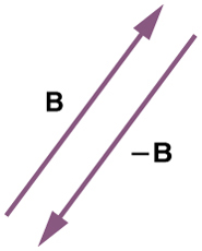
must first define what we mean by subtraction. The negative of a vector –B is defined to be B ; that is, graphically the negative of any vector has
the same magnitude but the opposite direction, as shown in Figure 3.20. In other words, B has the same length as –B , but points in the opposite direction. Essentially, we just flip the vector so it points in the opposite direction.
CHAPTER 3 | TWO-DIMENSIONAL KINEMATICS 93
Figure 3.20 The negative of a vector is just another vector of the same magnitude but pointing in the opposite direction. So B is the negative of –B ; it has the same length but opposite direction.
The subtraction of vector B from vector A is then simply defined to be the addition of –B to A . Note that vector subtraction is the addition of a negative vector. The order of subtraction does not affect the results.
(3.2)
A – B = A + (–B).
This is analogous to the subtraction of scalars (where, for example, 5 – 2 = 5 + (–2) ). Again, the result is independent of the order in which the
subtraction is made. When vectors are subtracted graphically, the techniques outlined above are used, as the following example illustrates.
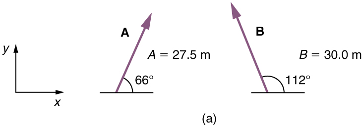
Example 3.2 Subtracting Vectors Graphically: A Woman Sailing a Boat
A woman sailing a boat at night is following directions to a dock. The instructions read to first sail 27.5 m in a direction 66.0º north of east from
her current location, and then travel 30.0 m in a direction 112º north of east (or 22.0º west of north). If the woman makes a mistake and
travels in the opposite direction for the second leg of the trip, where will she end up? Compare this location with the location of the dock.
Figure 3.21
Strategy
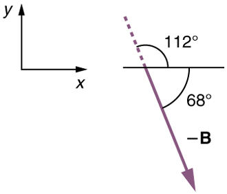
We can represent the first leg of the trip with a vector A , and the second leg of the trip with a vector B . The dock is located at a location
A + B . If the woman mistakenly travels in the opposite direction for the second leg of the journey, she will travel a distance B (30.0 m) in the
direction 180º – 112º = 68º south of east. We represent this as –B , as shown below. The vector –B has the same magnitude as B but is
in the opposite direction. Thus, she will end up at a location A + (–B) , or A – B .
Figure 3.22
We will perform vector addition to compare the location of the dock, A + B , with the location at which the woman mistakenly arrives,
A + (–B) .
94 CHAPTER 3 | TWO-DIMENSIONAL KINEMATICS
Solution
(1) To determine the location at which the woman arrives by accident, draw vectors A and –B .
(2) Place the vectors head to tail.
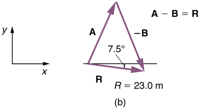
(3) Draw the resultant vector R .
(4) Use a ruler and protractor to measure the magnitude and direction of R .
Figure 3.23
In this case, R = 23.0 m and θ = 7.5º south of east.
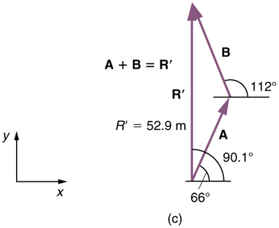
(5) To determine the location of the dock, we repeat this method to add vectors A and B . We obtain the resultant vector R' :
Figure 3.24
In this case R = 52.9 m and θ = 90.1º north of east.
We can see that the woman will end up a significant distance from the dock if she travels in the opposite direction for the second leg of the trip.
Discussion
Because subtraction of a vector is the same as addition of a vector with the opposite direction, the graphical method of subtracting vectors works
the same as for addition.
Multiplication of Vectors and Scalars
If we decided to walk three times as far on the first leg of the trip considered in the preceding example, then we would walk 3 × 27.5 m , or 82.5 m,
in a direction 66.0º north of east. This is an example of multiplying a vector by a positive scalar. Notice that the magnitude changes, but the
direction stays the same.
If the scalar is negative, then multiplying a vector by it changes the vector’s magnitude and gives the new vector the opposite direction. For example,
if you multiply by –2, the magnitude doubles but the direction changes. We can summarize these rules in the following way: When vector A is
multiplied by a scalar c ,
• the magnitude of the vector becomes the absolute value of c A ,
• if c is positive, the direction of the vector does not change,
• if c is negative, the direction is reversed.
In our case, c = 3 and A = 27.5 m . Vectors are multiplied by scalars in many situations. Note that division is the inverse of multiplication. For
example, dividing by 2 is the same as multiplying by the value (1/2). The rules for multiplication of vectors by scalars are the same for division; simply
treat the divisor as a scalar between 0 and 1.

CHAPTER 3 | TWO-DIMENSIONAL KINEMATICS 9