and
()
Example 1.33. Rectilinear motion
Problem : If the position of a particle along x – axis varies in time as :
Then :
1. What is the velocity at t = 0 ?
2. When does velocity become zero?
3. What is the velocity at the origin ?
4. Plot position – time plot. Discuss the plot to support the results obtained for the questions
above.
Solution : We first need to find out an expression for velocity by differentiating the given
function of position with respect to time as :
(i) The velocity at t = 0,
(ii) When velocity becomes zero :
For v = 0,
(iii) The velocity at the origin :
At origin, x = 0,
This means that particle is twice at the origin at t = 0.5 s and t = 1 s. Now,
Negative sign indicates that velocity is directed in the negative x – direction.

Figure 1.110. Position – time plot
We observe that slope of the curve from t = 0 s to t < 0.75 s is negative, zero for t = 0.75 and
positive for t > 0.75 s. The velocity at t = 0, thus, is negative. We can realize here that the
slope of the tangent to the curve at t = 0.75 is zero. Hence, velocity is zero at t = 0.75 s.
The particle arrives at x = 0 for t = 0.5 s and t = 1 s. The velocity at first arrival is negative as
the position falls on the part of the curve having negative slope, whereas the velocity at second
arrival is positive as the position falls on the part of the curve having positive slope.
Position - time plot
We use different plots to describe rectilinear motion. Position-time plot is one of them. Position
of the point object in motion is drawn against time. Evidently, it is a two dimensional plot. The
position is plotted with appropriate sign as described earlier.
Nature of slope
One of the important tool used to understand nature of such plots (as drawn above) is the slope of
the tangent drawn on the plot.In particular, we need to qualitatively ascertain whether the slope is
positive or negative. In this section, we seek to find out the ways to determine the nature of slope.
Mathematically, the slope of a straight line is numerically equal to trigonometric tangent of the
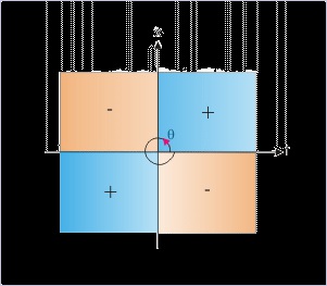
angle that the line makes with x – axis. It follows, therefore, that the slope of the straight line may
be positive or negative depending on the angle. It is seen as shown in the figure below, the tangent
of the angle in first and third quarters is positive, whereas it is negative in the remaining second
and fourth quarter. This assessment of the slope of the position - time plot helps us to identify
whether velocity is positive or negative?
Figure 1.111. Sign of the tangent of the angle
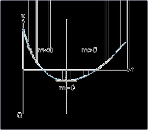
We may, however, use yet another simpler and effective technique to judge the nature of the
slope. This employs physical interpretation of the plot. We know that the tangent of the angle is
equal to the ratio of x (position) and t (time). In order to judge the nature of slope, we progress
with the time and determine whether “x” increases or decreases. The increase in “x” corresponds
to positive slope and a decrease, on the other hand, corresponds to negative slope. This assessment
helps us to quickly identify whether velocity is positive or negative?
Figure 1.112. Slope of the curve
Direction of motion
The visual representation of the curve might suggest that the tangent to the position – time plot
gives the direction of velocity. It is not true. It is contradictory to the assumption of the one
dimensional motion. Motion is either in positive or negative x – direction and not in any other
direction as would be suggested by the direction of tangent at various points. As a matter of fact,
the curve of the position – time plot is not the representation of the path of motion. The path of the
motion is simply a straight line. This distinction should always be kept in mind.
In reality, the nature of slope indicates the sense of direction, which can assume either of the two
possible directions. A positive slope of the curve denotes motion along the positive direction of
the referred axis, whereas negative slope indicates reversal of the direction of motion.
In the position – time plot as shown in the example at the beginning of the module (See Figure) ,
the slope of the curve from t = 0 s to t = 0.75 s is negative, whereas slope becomes positive for t
> 0.75 s. Clearly, an inversion of slope indicates reversal of direction. The particle, in the instant
case, changes direction once at t = 0.75 s during the motion.
Variation in the velocity
In addtion to the sense of direction, the position - time plot allows us to determine the magnitude
of velocity i.e. speed, which is equal to the magnitude of the slope. Here we shall see that the
position – time plot is not only helpful in determining magnitude and direction of the velocity, but
also in determining whether speed is increasing or decreasing or a constant.
Let us consider the plot generated in the example at the beginning of this module. The data set of
the plot is as given here :
t(s) x(m) Δx(m)
---------------------
0.0 1.0
0.1 0.72 -0.28
0.2 0.48 -0.24
0.3 0.28 -0.20
0.4 0.12 -0.16
0.5 0.00 -0.12
0.6 -0.08 -0.08
0.7 -0.12 -0.12
0.8 -0.12 0.00
0.9 -0.08 0.04
1.0 0.00 0.08
1.1 0.12 0.12
1.2 0.28 0.16
---------------------
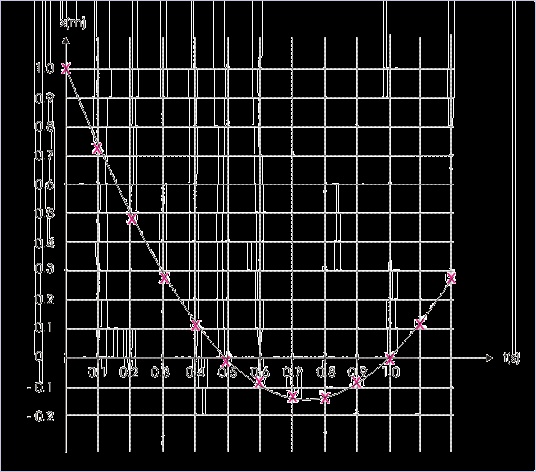
In the beginning of the motion starting from t = 0, we see that particle covers distance in
decreasing magnitude in the negative x - direction. The magnitude of difference, Δx, in equal time
interval decreases with the progress of time. Accordingly, the curve becomes flatter. This is
reflected by the fact that the slope of the tangent becomes gentler till it becomes horizontal at t =
0.75 s. Beyond t = 0.75 s, the velocity is directed in the positive x – direction. We can see that
particle covers more and more distances as the time progresses. It means that the velocity of the
particle increases with time and the curve gets steeper with the passage of time.
Figure 1.113. Position – time plot
In general, we can conclude that a gentle slope indicates smaller velocity and a steeper slope
indicates a larger velocity.
Velocity - time plot
In general, the velocity is a three dimensional vector quantity. A velocity – time would, therefore,
require additional dimension. Hence, it is not possible to draw velocity – time plot on a three
dimensional coordinate system. Two dimensional velocity - time plot is possible, but its drawing
is complex.
One dimensional motion, having only two directions – along positive or negative direction of axis,
allows plotting velocity – time graph. The velocity is treated simply as scalar speed with one
qualification that velocity in the direction of chosen reference is considered positive and velocity
in the opposite direction to chosen reference is considered negative.
In "speed- time" and "velocity – time" plots use the symbol “v” to represent both speed and
velocity. This is likely to create some confusion as these quantities are essentially different.
We use the scalar symbol “v” to represent velocity as a special case for rectilinear motion,
because scalar value of velocity with appropriate sign gives the direction of motion as well.
Therefore, the scalar representation of velocity is consistent with the requirement of
representing both magnitude and direction. Though current writings on the subject allows
duplication of symbol, we must, however, be aware of the difference between two types of
plot. The speed (v) is always positive in speed – time plot and drawn in the first quadrant of
the coordinate system. On the other hand, velocity (v) may be positive or negative in velocity
– time plot and drawn in first and fourth quadrants of the two dimensional coordinate system.
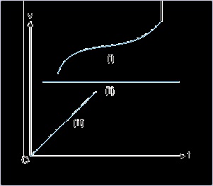
The nature of velocity – time plot
Velocity – time plot for rectilinear motion is a curve (Figure i). The nature of the curve is
determined by the nature of motion. If the particle moves with constant velocity, then the plot is a
straight line parallel to the time axis (Figure ii). On the other hand, if the velocity changes with
respect to time at uniform rate, then the plot is a straight line (Figure iii).
Figure 1.114. Velocity – time plot
The representation of the variation of velocity with time, however, needs to be consistent with
physical interpretation of motion. For example, we can not think of velocity - time plot, which is a
vertical line parallel to the axis of velocity (Figure ii). Such plot is inconsistent as this would
mean infinite numbers of values, against the reality of one velocity at a given instant. Similarly,
the velocity-time plot should not be intersected by a vertical line twice as it would mean that the
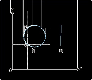


particle has more than one velocity at a given time (Figure i).
Figure 1.115. Velocity – time plot
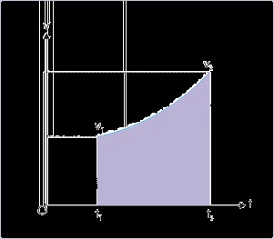
Area under velocity – time plot
The area under the velocity – time plot is equal to displacement. The displacement in the small
time period “dt” is given by :
Integrating on both sides between time intervals
The right hand side integral graphically represents an area on a plot drawn between two variables :
velocity (v) and time (t). The area is bounded by (i) v-t curve (ii) two time ordinates t 1 and t 2 and
(iii) time (t) axis as shown by the shaded region on the plot. Thus, the area under v-t plot bounded
by the ordinates give the magnitude of displacement (Δx) in the given time interval.
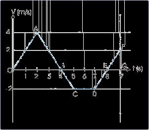

Figure 1.116. Area under velocity – time plot
When v-t curve consists of negative values of velocity, then the curve extends into fourth quadrant
i.e. below time axis. In such cases, it is sometimes easier to evaluate area above and below time
axis separately. The area above time axis represents positive displacement, whereas area under
time axis represents negative displacement. Finally, areas are added with proper sign to obtain the
net displacement during the motion.
To illustrate the working of the process for determining displacement, let us consider the
rectilinear motion of a particle represented by the plot shown.
Figure 1.117. Velocity – time plot
Here,
A switch from positive to negative value of velocity and vice-versa is associated with change of
direction of motion. It means that every intersection of the v – t curve with time axis represents a
reversal of direction. Note that it is not the change of slope (from postive to negative and and vive
versa) like on the position time that indicates a change in the direction of motion; but the
intersection of time axis, which indicates change of direction of velocity. In the motion described
in figure above, particle undergoes reversal of direction at two occasions at B and E.
It is also clear from the above example that displacement is given by the net area (considering
appropriate positive and negative sign), while distance covered during the motion in the time
interval is given by the cumulative area without considering the sign. In the above example,
distance covered is :

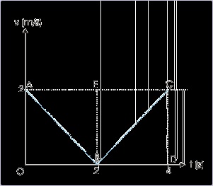


s = Area of triangle OAB + Area of trapezium BCDE + Area of triangle EFG
A person walks with a velocity given by |t – 2| along a straight line. Find the distance and
displacement for the motion in the first 4 seconds. What is the average velocity in this period?
Here, the velocity is equal to the modulus of a function in time. It means that velocity is always
positive. An inspection of the function reveals that velocity linearly decreases for the first 2
second from 2 m/s to zero. It, then, increases from zero to 2 m/s in the next 2 seconds. In order to
obtain distance and displacement, we draw the Velocity – time plot plot as shown.
The area under the plot gives displacement. In this case, however, there is no negative
displacement involved. As such, distance and displacement are equal.
Figure 1.117. Velocity – time plot
and the average velocity is given by :
Uniform motion
Uniform motion is a subset of rectilinear motion. It is the most simplified class of motion. In this

case, the body under motion moves with constant velocity. It means that the body moves along a
straight line without any change of magnitude and direction as velocity is constant. Also, a
constant velocity implies that velocity is constant all through out the motion. The velocity at
every instant during motion is, therefore, same.
It follows then that instantaneous and averages values of speed and velocity are all equal to a
constant value for uniform motion :
The motion of uniform linear motion has special significance, as this motion exactly echoes the
principle enshrined in the first law of motion. The law states that all bodies in the absence of
external force maintain their speed and direction. It follows, therefore, that the study of uniform
motion is actually the description of motion, when no external force is in play.
The absence of external force is hypothetical in our experience as bodies are always subject to
external force(s). The force of gravitation is short of omnipresent force that can not be overlooked
- atleast on earth. Nevertheless, the concept of uniform motion has great theoretical significance
as it gives us the reference for the accelerated or the non-uniform real motion.
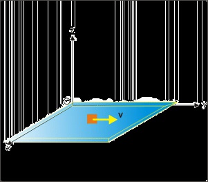
On the earth, a horizontal motion of a block on a smooth plane approximates uniform motion as
shown in the figure. The force of gravity acts and normal reaction force at the contact between
surfaces act in vertically, but opposite directions. The two forces balances each other. As a result,
there is no net force in the vertical direction. As the surface is smooth, we can also neglect
horizontal force due to friction, which could have opposed the motion in horizontal direction. This
situation is just an approxmiation for we can not think of a flawless smooth surface in the first
place; and also there would be intermolecular attraction between the block and surface at the
contact. In brief, we can not achieve zero friction - eventhough the surfaces in contact are
perfectly smooth. However, the approximation like this is helpful for it provides us a situation,
which is equivalent to the motion of an object without any external force(s).
Figure 1.118. Uniform motion
We can also imagine a volumetric space, where massive bodies like planets and stars are not
nearby. The motion of an object in that space, therefore, would be free from any external force and
the motion would be in accordance with the laws of motion. The study of astronauts walking in the
space and doing repairs to the spaceship approximates the situation of the absence of external
force. The astronaut in the absence of the force of gravitation and friction (as there is no
atmosphere) moves along with the velocity of the spaceship.
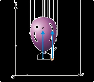
Motion of separated bodies
The fact that the astronauts moves with the velocity of spaceship is an important statement about
the state of motion of the separated bodies. A separated body acquires the velocity of the
containing body. A pebble released from a moving train or dropped from a rising balloon is an
example of the motion of separated body. The pebble acquires the velocity of the train or the
balloon as the case may be.
Figure 1.119. Motion of separated bodies
It means that we must assign a velocity to the released body, which is equal in magnitude and
direction to that of the body from which the released body has separated. The phenomena of
imparting velocity to the separated body is a peculiarity with regard to velocity. We shall learn
that acceleration (an attribute of non-uniform motion) does not behave in the same fashion. For
example, if the train is accelerating at the time, the pebble is dropped, then the pebble would not
acquire the acceleration of the containing body.
The reason that pebble does not acquire the acceleration of the train is very simple. We know that
acceleration results from application of external force. In this case, the train is accelerated as the
engine of the train pulls the compartment (i.e. applies force on the compartment. The pebble,
being part of the compartment), is also accelerated till it is held in the hand of the passenger.
However, as the pebble is dropped, the connection of the pebble with the rest of the system or with
the engine is broken. No force is applied on the pebble in the horizontal direction. As such, pebble
after being dropped has no acceleration in the horizontal direction.
In short, we can conclude that a separated body acquires velocity, but not the acceleration.
1.17. Rectilinear motion (application)*
Questions and their answers are presented here in the module text format as if it were an extension
of the treatment of the topic. The idea is to provide a verbose explanation, detailing the
application of theory. Solution presented is, therefore, treated as the part of the understanding
process – not merely a Q/A session. The emphasis is to enforce ideas and concepts, which can not
be completely absorbed unless they are put to real time situation.
Representative problems and their solutions
We discuss problems, which highlight certain aspects of rectilinear motion. The questions are
categorized in terms of the characterizing features of the subject matter :
Interpretation of position - time plot
Interpretation of displacement - time plot
Displacement
Average velocity
Position vector
Example 1.34.
Problem : Two boys (P and Q) walk to their respective school from their homes in the
morning on a particular day. Their motions are plotted on a position – time graph for the day
as shown. If all schools and homes are situated by the side of a straight road, then answer the
followings :
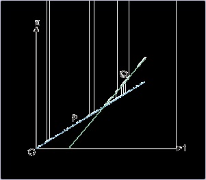
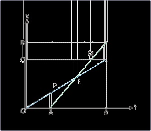
Figure 1.120. Motion of two boys
Position – time plot of a rectilinear motion.
1. Which of the two resides closer to the school?
2. Which of the two starts earlier for the school?
3. Which of the two walks faster?
4. Which of the two reaches the school earlier?
5. Which of the two overtakes other during walk?
Solution : In order to answer questions, we complete the drawing with vertical and horizontal
lines as shown here. Now,
Figure 1.121. Motion of two boys
Position – time plot of a rectilinear motion.
1: Which of the two resides closer to the school?
We can answer this question by knowing the displacements. The total displacements here are
OC by P and OD by Q. From figure, OC < OD. Hence, P resides closer to the school.
2: Which of the two starts earlier for the school?
The start times are point O for P and A for Q on the time axis. Hence, P starts earlier for
school.
3: Which of the two walks faster?
The speed is given by the slope of the plot. Slope of the motion of P is smaller than that of Q.
Hence, Q walks faster.
4: Which of the two reaches the school earlier?
Both boys reach school at the time given by point B on time axis. Hence, they reach school at
the same time.
5: Which of the two overtakes other during walk?
The plots intersect at a point E. They are at the same location at this time instant. Since, speed
of B is greater, he overtakes A.
Interpretation of displacement - time plot
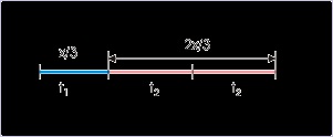
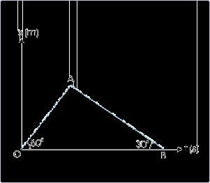
Example 1.35.
Problem : A displacement – time plot in one dimension is as shown. Find the ratio of
velocities represented by two straight lines.
Figure 1.122. Displacement-time plot
There two segments of different velocities.
Solution : The slope of displacement – time plot is equal to velocity. Let v1 and v2 be the
velocities in two segments, then magnitudes of velocities in two segments are :


We note that velocity in the first segment is positive, whereas velocity in the second segment
is negative. Hence, the required ratio of two velocities is :
Displacement
Example 1.36.
Problem : The displacement “x” of a particle moving in one dimension is related to time “t”
as :
where “t” is in seconds and “x” is in meters. Find the displacement of the particle when its
velocity is zero.
Solution : We need to find “x” when velocity is zero. In order to find this, we require to have
an expression for velocity. This, in turn, requires an expression of displacement in terms of
time. The given expression of time, therefore, is required to be re-arranged :
Squaring both sides, we have :
Now, we obtain the required expression of velocity in one dimension by differentiating the
above relation with respect to time,
According to question,
Putting this value of time in the expression of displacement, we have :
Average velocity
Example 1.37.