Once it becomes necessary to include more than two state variables in a model, and if the interactions are nonlinear, the analytical and phase plane techniques can no longer be used. This section will consider several higher-order models and use digital simulation as the tool for analysis. The first example will be a rather logical extension of some of our earlier population models.
| A. Population Models with Age Specific Birth and Death Rates |
Even cursory examination of the assumptions behind the population model assumed in Section IV show them to be unrealistic. The model

assumes r to be the difference between the birth rate and death rate, and that these rates are not a function of time or population.
An improvement on this model would allow different birth and death rates to be assigned to members of the population of different ages. This means that the population will have to be divided into groups with similar rates, and that the number of groups necessary will be the number of state variables required. ???
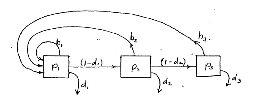
For example, let p1 be the population of people between zero
and ten years of age, p2 the population of those from eleven to
twenty, p3 those from twenty-one to thirty, etc.
Let b1 be the average birth rate of  , and b2 the rate for
  , etc., with d1 being the average
death rate of
, etc., with d1 being the average
death rate of  , etc.
Assume the maximum possible age to be one hundred.
The equations for this model are given by
, etc.
Assume the maximum possible age to be one hundred.
The equations for this model are given by

where the time interval represented by each successive value of n is the same as that for the age span for each population group, i.e., ten years. Likewise, the birth and death rate are numbers per ten-year period. The equations in Equation 8.2 can be described by a flow graph, illustrated below for only three sections.
These equations can be easily programmed and solved on a computer, but because they are linear, there are some interesting properties that can be worked out analytically. They are best seen by writing ??? as a matrix equation.

In compact vector notation, this becomes

>From this expression, it is easily seen that the population
distribution after n times ten years from some initial population
distribution  is given by

There are several interesting observations for the readers with a
knowledge of matrix theory.
After several steps of  , the age distribution will assume a form
given by the eigenvector of the largest eigenvalue of
, the age distribution will assume a form
given by the eigenvector of the largest eigenvalue of  .
.
After several steps, the age distribution will stop changing and this eigenvector is called the stable age distribution, and this largest eigenvalue is the stable growth rate if the eigenvalue is greater than one (decay rate if is is less than one). The problem is a bit more complicated if the eigenvalues are complex (where oscillations occur).
It is possible to modify the equations of Equation 8.2 to allow for shorter T
in Euler's method than the span of ages in a population group, and to
allow different spans for different groups. Let T be the time
interval between each calculation of new levels. Let Si be the span
of ages for the group  . Consider the population group
 . During one time interval
  , the number that dies is
 , the fraction that advances to the next group is
 times those that do not die
  , and the rest
  stay in the group.
The equations become
stay in the group.
The equations become


The birth rates bi are the number of births per initial value
of population in a group pi per time interval  .
The death rate is likewise per time interval
.
The death rate is likewise per time interval  .
.
This is a rather general formulation that allows non-equal age grouping and short time interval without requiring a high order. The system can be posed in matrix form as before. The main limitation on this approach is that it is linear. In general, the various birth and death rates will depend on crowding and other environmental and social factors that are assumed constant here. Even so, insight can be gained into population growth by experiments on these simple linear models.
| B. A Model of the World |
One of the most interesting and controversial applications of dynamic modeling is the work of J. Forrester at Massachusetts Institute of Technology on a simulation of the world. In 1970 at the request of an international group called the Club of Rome, Forrester developed a fifth-order model of the work using what he calls "system dynamics," methods that had previously only been applied to industrial and urban systems. The preliminary results were published 1 in 1971, and further work done by his colleague Dennis Meadows was published 2 in 1972. The response to this work was incredible. There has been a flood of articles in newspapers, popular magazines, and scholarly journals – some in praise and others in condemnation. Most have been superficial and emotional. There is, however, one interesting serious response published by a group in England 3 in 1973.
The state variables chosen by Forrester are:
| N | population |
| C | capital |
| A | agriculture |
| P | pollution |
| R | non-renewable resources |
The model then assumed the form

In one sense, this work is a logical extension of the dynamic modeling discussed in the earlier sections of this paper, and Forrester's formalism is nothing more than using Euler's method to solve simultaneous differential equations. In another sense, his bold use of these methods represents a distinct departure from the specialized models that the demographer, economist, etc. have used in their separate disciplines.
There are several features of Forrester's approach that should be
understood. The functions  ,
,  , etc. are developed in
a complicated way using the theories and empirical results of specialists
in those areas. This generally means that there are numerous intermediate
variables defined and used, both for insight and because the data occurs
that way. One should not confuse these with the state variables, however.
Forrester also uses tables rather than functions to implement the fi
in the simulation. These are usually easier to handle by
non-mathematicians, and again in the form that empirical relations are
often known.
, etc. are developed in
a complicated way using the theories and empirical results of specialists
in those areas. This generally means that there are numerous intermediate
variables defined and used, both for insight and because the data occurs
that way. One should not confuse these with the state variables, however.
Forrester also uses tables rather than functions to implement the fi
in the simulation. These are usually easier to handle by
non-mathematicians, and again in the form that empirical relations are
often known.
A version of the world model has been programmed in APL on an IBM 370 at Rice. The details of this program and instructions on its use are included in the appendix. Examples of the results of the model are given in 1 and 2 and a criticism in 3.
J.W. Forrester. (1971). World Dynamics. Cambridge: Wright-Allen Press.
D.L. Meadows, et al. (1972). The Limits to Growth. New York: Universe Books.
H.S.D. Cole, et. al. (1973). Models of Doom- A Critique of the Limits to Growth. New York: Universe Books.
T.R. Malthus, L.F. Richardson. (1956). Mathematics of Population and Food, and Mathematics of War and Foreign Politics. [edited by J.R. Newman, and Simon and Schuster]. The World of Mathematics, 2,