In the last few sections, we discussed first-order models of various systems and studied the types of interactions that could be modeled and the nature of the solutions of these models. Of the several indicated generalizations that could be made, this section will consider adding another state variable, so that the effects of two interacting variables can be used and studied. This will greatly increase the class of systems we can model and the class of solutions that result. In addition, a very interesting set of classical problems fall into this class with interesting solutions and interpretations.
To illustrate the general problem, consider a system that contains populations of two different types with distinctly different characteristics. Assume these two populations have a strong effect on each other, as well as being influenced differently by their environment, so that modeling them by a single total population would not yield useful results. We must, therefore, have two separate state variables to describe the systems, and this could perhaps be done in the following way.


Here the rate of change of population p1 is assumed to depend
on both the populations p1 and  ;
and likewise, the rate of change of p2 is assumed to depend
on p1 and
;
and likewise, the rate of change of p2 is assumed to depend
on p1 and  , but in perhaps a different way.
Many types of interactions could be considered.
It might be that p1 and p2 compete for the same
source of food or resources;
it might be that p1 is a prey of the predator  ;
or it could be that they both contribute to the welfare of the other.
These assumptions would be implemented in the choice
of
;
or it could be that they both contribute to the welfare of the other.
These assumptions would be implemented in the choice
of  and
and  to describe the particular case.
The best known classical models of these types were proposed by
Lotka (1925)
and
Volterra (1926).
Later,
Gause (1934)
did further experimental and interpretative work.
Most of this type of work was done in population ecology.6, 1.
to describe the particular case.
The best known classical models of these types were proposed by
Lotka (1925)
and
Volterra (1926).
Later,
Gause (1934)
did further experimental and interpretative work.
Most of this type of work was done in population ecology.6, 1.
| A. The Simple Lotka-Volterra Competition Model |
Consider the particular for for the two-variable model to be


This might be a simple model of two competing populations, where a and c are the net rate of increase that would occur if the other population did not exist. The coefficients b and d model the negative effects of interaction on the rates of change as a measure of how often one encounters the other.
To simplify the mathematics, a change of variables will be made. Consider the rearrangement of Equation 7.3 into


Now let  and
and
 then, Equation 7.5 becomes


Note that x and y are related to p1 and p2 by
simple constant
multipliers or scale factors, and therefore, the nature of the solution
of Equation 7.7 is the same as Equation 7.3, but now there are only two
parameters, a and  , to consider.
In fact, by allowing a change of scale of the time variable, it is
possible to reduce the number of parameters to one, but we will not do
that.
The problem of solving the coupled equation of Equation 7.7 or, more generally,
of Equation 7.1 can be approached three ways.
In some cases, an analytical equation for the solution can be found.
This is always true if the equations are linear, but unfortunately,
almost never true if they are nonlinear.
Another approach was the phase plane where one solution is plotted as a
function of the other, with time as an implicit variable.
Very important characteristics of the solution can often be determined
by phase plane methods without actually finding the solution.
Finally, the equations can be numerically solved by simulation on a
digital computer using Euler's method or some other more efficient
algorithm.
, to consider.
In fact, by allowing a change of scale of the time variable, it is
possible to reduce the number of parameters to one, but we will not do
that.
The problem of solving the coupled equation of Equation 7.7 or, more generally,
of Equation 7.1 can be approached three ways.
In some cases, an analytical equation for the solution can be found.
This is always true if the equations are linear, but unfortunately,
almost never true if they are nonlinear.
Another approach was the phase plane where one solution is plotted as a
function of the other, with time as an implicit variable.
Very important characteristics of the solution can often be determined
by phase plane methods without actually finding the solution.
Finally, the equations can be numerically solved by simulation on a
digital computer using Euler's method or some other more efficient
algorithm.
| B. The Phase Plane |
The pair of equations in Equation 7.1 can be reduced to a single equation by
eliminating the time variable  .
This can be done by simply dividing one by the other to give
.
This can be done by simply dividing one by the other to give

The solution of this equation is examined in
the  plane, which is called the
phase plane.
plane, which is called the
phase plane.
As an example, consider the competition model in Equation 7.7 in the phase plane

Solutions in the phase plane are
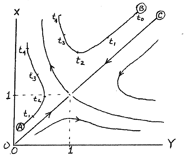
The trajectory starting at A gives the value of x and y with
time  , an implicit variable, indicated by the values shown. If a different initial mixture of populations had been assumed,
e.g.,
, an implicit variable, indicated by the values shown. If a different initial mixture of populations had been assumed,
e.g.,  , then a different trajectory would result.
Indeed, any initial mixture is a point on the phase plane, and the
trajectories indicate how they evolve in time.
The more conventional time solutions are shown for the initial
of A by
, then a different trajectory would result.
Indeed, any initial mixture is a point on the phase plane, and the
trajectories indicate how they evolve in time.
The more conventional time solutions are shown for the initial
of A by
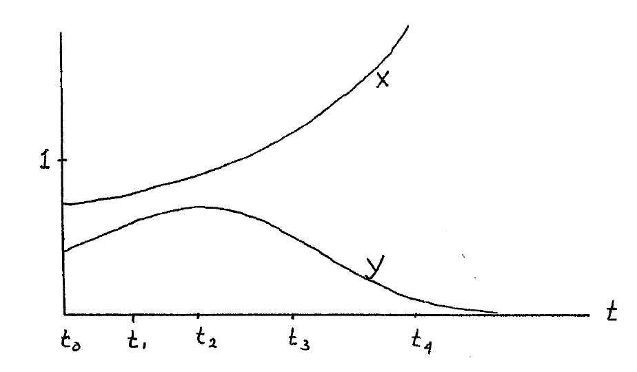
and for B by
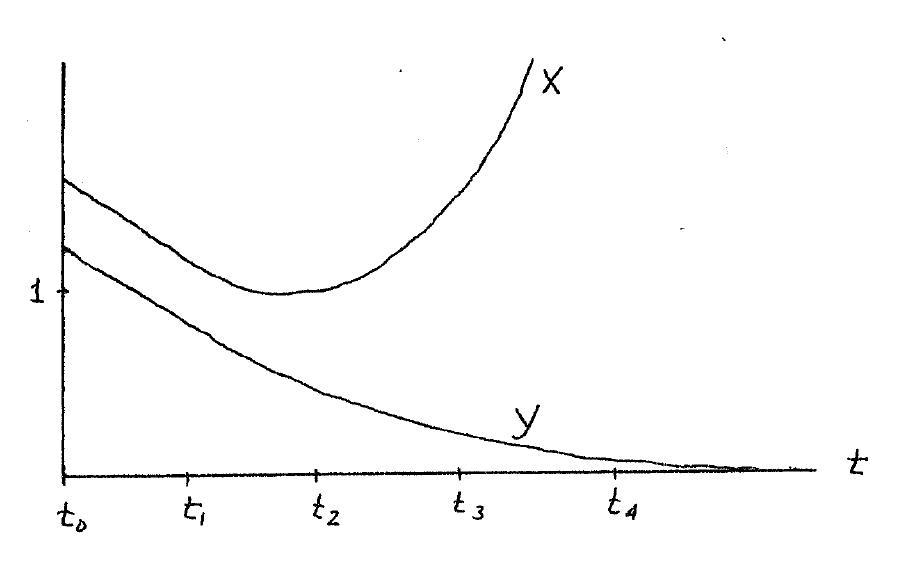
Note the relation of the phase plane plots and the time plots. This particular problem will later be examined in greater detail.
One might wonder why this peculiar representation of the solutions is the form of one variable considered as a form of the other. This phase plane approach, although a bit unnatural at first, proves to be a very powerful tool. It is used by many in the literature 6 10 1 2 and is a standard mathematical tool. 8 9 It is worthwhile developing this concept before analyzing several physical systems.
Note that the phase plane contains all possible time plane plots for various mixtures. It can be shown that if the system has unique solutions, then the phase plane trajectories cannot cross. This means that a few key trajectories can be constructed which will make obvious what all other trajectorie will have to be. For example, in the above competition model, the initial mixture always determines who the eventual winner will be. Any initial mixture to the right of the line from the origin to C results in y increasing without bound and x becoming extinct. Initial mixture to the left gives the opposite result.
There are several procedures that aid in the construction and
interpretation of phase plane trajectories.
There are special points on the plane known as
equilibrium points or
singular points that are important.
If both  and
and  in ??? are zero,
then x and y are
constants and the system is in equilibrium.
This means that at these points both the numerator and denominator of
Equation 7.9 are zero.
For the competition model of Equation 7.10, there is a singular point
at
in ??? are zero,
then x and y are
constants and the system is in equilibrium.
This means that at these points both the numerator and denominator of
Equation 7.9 are zero.
For the competition model of Equation 7.10, there is a singular point
at  and
and  , and another
at
, and another
at  and
and  .
Singular points may be stable or unstable depending on whether small
perturbations away from the point tend back to it or go away from it. Both points mentioned above are unstable.
.
Singular points may be stable or unstable depending on whether small
perturbations away from the point tend back to it or go away from it. Both points mentioned above are unstable.
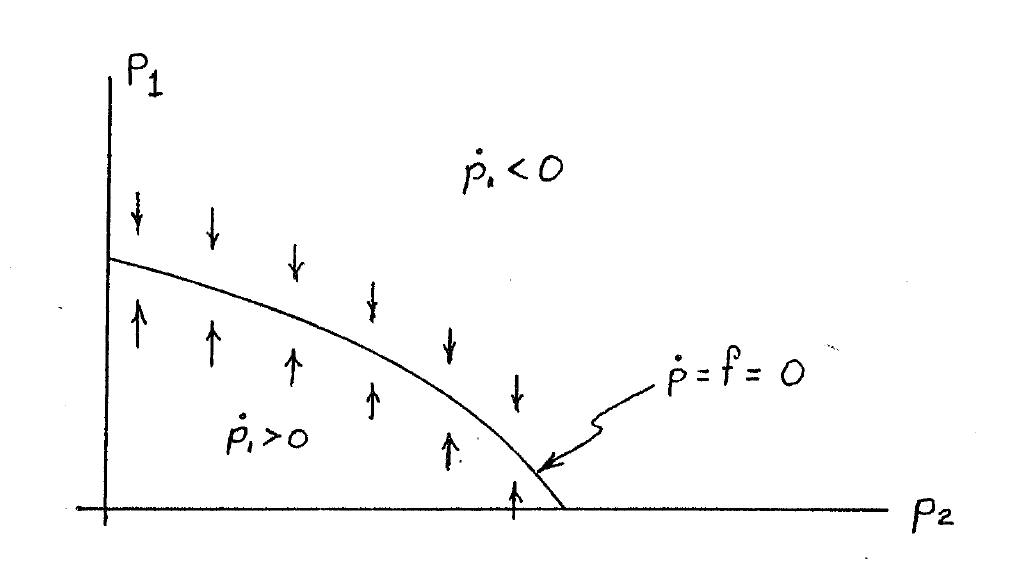
A particular informative way of finding the singular or equilibrium points is to consider what are called partial equilibrium lines in the phase plane. The curve of all possible solutions of the equition

is called the
partial equilibrium curve for population  .
This is understood by considering the first equation in Equation 7.1 alone.
The equation Equation 7.11 implies
.
This is understood by considering the first equation in Equation 7.1 alone.
The equation Equation 7.11 implies  , therefore,
one side of this curve
, therefore,
one side of this curve  will be positive and on
the other side it will be negative.
If a particular
will be positive and on
the other side it will be negative.
If a particular  curve was given by
for any given fixed  , p1 would move to
the
, p1 would move to
the  partial equilibrium curve.
This curve would, therefore, give the effects of p2 on the
equilibrium values of
partial equilibrium curve.
This curve would, therefore, give the effects of p2 on the
equilibrium values of  .
In other words, for a system controlled by the first equation of Equation 7.1
if p2 is given, the
.
In other words, for a system controlled by the first equation of Equation 7.1
if p2 is given, the  curve will give the equilibrium
value psub1 approaches.
.pp
In fact, however, p2 is not fixed, but must obey the second
equation in Equation 7.1.
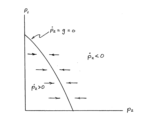
If this equation is examined separately, we have a second curve called
the partial equilibrium curve
for p2 given by
curve will give the equilibrium
value psub1 approaches.
.pp
In fact, however, p2 is not fixed, but must obey the second
equation in Equation 7.1.
If this equation is examined separately, we have a second curve called
the partial equilibrium curve
for p2 given by

A similar analysis of this equation shows the effects of p1 on the equilibrium values of p2, and can be visualized by the following illustration of a g=0 curve.
If these two curves are considered simultaneously, then not only are
the singular points determined by the intersections, but the stability
of the points and the nature and direction of the trajectories can be
estimited by the signs of  and
and  in the
various regions.
For these illustrated curves of f=0 and g=0, we have
in the
various regions.
For these illustrated curves of f=0 and g=0, we have
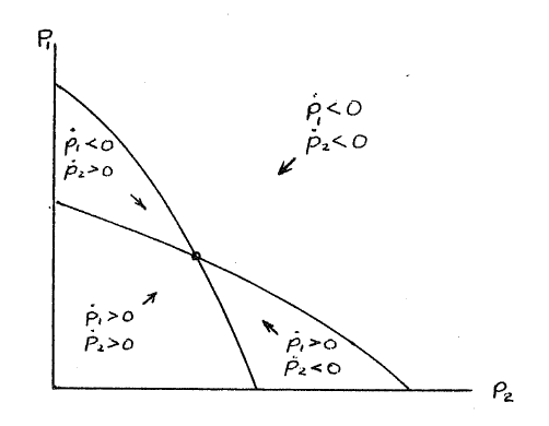
This determines the singular point, and the directions show that it is stable. Applying this to the Lotka-Volterra competition model of Equation 7.7 for the partial equilibrium curves gives

or

and

or

In the phase plane, these are
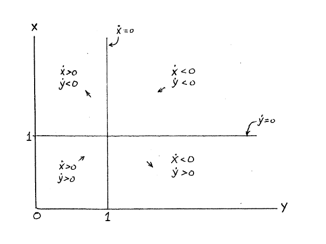
Another tool that is very useful and is related to the preceding
discussion is the method of isoclines.8???
Here we find curves in the phase plane where all the trajectories that
cross that curve have the same slope.
The partial equilibrium curves are two isoclines.
The  curve implies from Equation 7.9 that the slope of all
trajectories along that curve is zero.
The slope of all trajectories along the
curve implies from Equation 7.9 that the slope of all
trajectories along that curve is zero.
The slope of all trajectories along the  curve is infinite.
If we find the isocline for a slope of
curve is infinite.
If we find the isocline for a slope of  , this is done from Equation 7.9 by
setting
, this is done from Equation 7.9 by
setting

For the competition model with  , we have

Solving for x as a function of y gives

The  isocline is
  . The
. The  isocline
is
isocline
is  . The
. The  isocline is

and  gives
gives

In the phase plane the isocline looks like
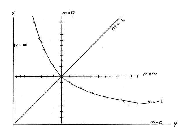
Note how the isoclines aid one in sketching or visualizing the phase plane solution trajectories.
This should be enough detail on this approach to allow application to the various two-variable models that can be so interesting.
| C. : Competition Models |
We will now return to the competition model of Equation 7.3 and examine it in
more detail.
Consider a situation where the uninhibited growth rate of
population p