Since it is the dynamic nature of a system that we want to model and understand, the simplest form will be considered. This will involve one state variable and will give rise to so-called "exponential" growth.
First consider a mathematical model of a bank savings account. Assume
that there is an initial deposit but after that, no deposits or
withdrawals. The bank has an interest rate ri and service charge
rate rs that are used to calculate the interest and service charge
once each time period. If the net income (interest less service charge)
is re-invested each time, and each time period is denoted by the integer
 , the future amount of money could be calculated from

A net growth rate r is defined as the difference

and this is further combined to define R by

The basic model in Equation 4.1 simplifies to give


This equation is called a
first-order difference equation, and the solution M(n) is found in a
fairly straightforward way. Consider the equation for the first few
values of 


The solution to Equation 4.4 is a geometric sequence that has an initial value of
M(0) and increases as a function of n if R is greater than 1
 , and decreases toward zero as a function of n if R is
less than 1
, and decreases toward zero as a function of n if R is
less than 1  . This makes intuitive sense. One's account
grows rapidly with a high interest rate and low service charge rate, and
would decrease toward zero if the service charges exceeded the interest.
. This makes intuitive sense. One's account
grows rapidly with a high interest rate and low service charge rate, and
would decrease toward zero if the service charges exceeded the interest.
A second example involves the growth of a population that has no
constraints. If we assume that the population is a continuous function of
time  , and that the birth rate rb and death rate rd
are constants (
, and that the birth rate rb and death rate rd
are constants ( not functions of the population p(t) or time
  ), then the rate of increase in population can be written

There are a number of assumptions behind this simple model, but we delay those considerations until later and examine the nature of the solution of this simple model. First, we define a net rate of growth

which gives

which is a first-order linear differential equation. If the value of the
population at time equals zero is  , then the solution of Equation 4.14 is
given by
, then the solution of Equation 4.14 is
given by

The population grows exponentially if r is positive (if  ) and decays exponentially if r is negative (
 ). The fact that Equation 4.15 is a solution of Equation 4.14 is easily verified by
substitution. Note that in order to calculate future values of
population, the result of the past as given by p(0) must be known.
(
). The fact that Equation 4.15 is a solution of Equation 4.14 is easily verified by
substitution. Note that in order to calculate future values of
population, the result of the past as given by p(0) must be known.
( is a state variable and only one is necessary.)
It is worth spending a bit of time considering the nature of the solution of the difference Equation 4.4 and the differential Equation 4.14. First, note that the solutions of both increase at the same "rate". If we sample the population function p(t) at intervals of T time units, a geometric number sequence results. Let pn be the samples of p(t) given by

This give for Equation 4.15

which is the same as ??? if

This means that one can calculate samples of the exponential solution of differential equations exactly by solving the difference Equation 4.4 if R is chosen by Equation 4.18. Since difference equations are easily implemented on a digital computer, this is an important result; unfortunately, however, it is exact only if the equations are linear. Note that if the time interval T is small, then the first two terms of the Taylor's series give

which is somewhat similar to Equation 4.3. Another view of the relation can be seen by approximating Equation 4.14 by

which gives


having a solution

This implies Equation 4.21 also, and the method is known as Euler's method for numerically solving a differential equation.
These approximations are used often in modeling. For population models a differential evuation is often used, even though it is obvious that births and deaths occur at random discrete times and populations can take on only integer values. The approximation makes sense only if we use large aggregates of individuals. We end up modeling a process that occurs at random discrete points in time by a continuous time mode, which is then approximated by a uniformly-spaced discrete time difference equation for solution on a digital computer!
The rapidity of increase of an exponential is usually surprising and it is this fact that makes understanding it important. There are several ways to describe the rate of growth.


This states that r is the rate of growth per unit of  . For
example, the growth rate for the U.S. is about 0.014 per year, or an
increase of 14 people per thousand people each year.
. For
example, the growth rate for the U.S. is about 0.014 per year, or an
increase of 14 people per thousand people each year.
Another measure of the rate is the time for the variable to double in
value. This doubling time,  , is constant and can easily be shown
to be given by
, is constant and can easily be shown
to be given by

For example, doubling times for several rates are given by
| r | Td |
| .01 | 70 |
| .02 | 35 |
| .03 | 23 |
| .04 | 17 |
| .05 | 14 |
| .06 | 12 |
The present world population is about three billion, and the growth rate is 2.1% per year. This gives

with p(t) measured in billions of people and t in years. This gives a doubling time of 33 years. While it is easy to talk of growth rate and doubling times, these have real predictive meaning only if the growth is exponential.
There are two rather different approaches that can be used when describing some physical phenomenon by exponential growth. It can be viewed as an empirical description of how some variables tend to evolve in time. This is a data-fitting view that is pragmatic and flexible, but does not give much insight or direction on how to conduct experiments or what other things might be implied.
The second approach primarily considers the underlying differential equation as a "law" of growth that results in exponential behavior. This law has various assumptions and implications that can be examined for reasonableness or verified by independent experiment. While perhaps not so important for the first-order linear equation here, this approach becomes necessary for the more complicated models later.
These approaches must often be mixed. The data will imply a model or equation which will give direction as to what data should be taken, which will in turn imply modifications, etc. The process where structure is chosen and the parameters are chosen so that the model solution agrees with observed data is a form of parameter identification. That was how Equation 4.28 was determined.
When examining data that has been plotted in fashion, it is often hard to say much about its basic nature. For example if a time series is plotted on linear coordinates as follows
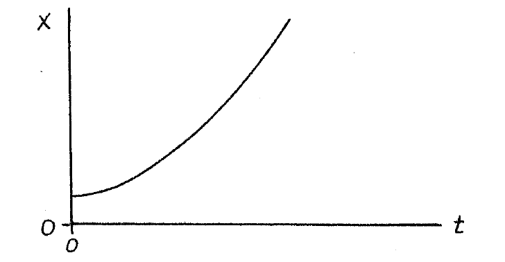
it would not be obvious if it were samples of an exponential, a parabola, or some other function. Straight lines, on the other hand, are easy to identify and so we will seek a method of displaying data that will use straight lines.
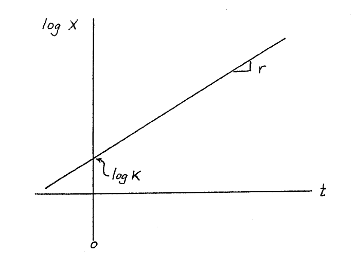
If x(t) is an exponential, then

Taking logarithms of base e for both sides of Equation 4.29 gives

If, rather than plotting x versus  , we plot the log of x
versus
, we plot the log of x
versus  , then we have a straight line with a slope of r and an
intercept of log
, then we have a straight line with a slope of r and an
intercept of log  . It would look like
Actually using the logarithm of a variable is awkward so the variable itself can be plotted on logarithmic coordinates to give the same result. Graph paper with logarithmic spacing along one coordinate and uniform spacing along the other is called semi-log paper.
Consider the plot of the U.S. population displayed on semi-log paper in Figure 3. Note that there were two distinct periods of exponential growth, one from 1600 to 1650, and another from 1650 to 1870. To calculate the growth rate over the 1650 – 1870 period, we can calculate the slope.


During that period, there was a 3% per year growth rate or, in other terms, a 23-year doubling time.
An alternative is to measure the doubling time and calculate r from Equation 4.27. Still another approach is to measure the time necessary for the population to increase by e=2.72... The growth rate is the reciprocal of that time interval. Derive and check these for yourself.
The data displayed in Figures 1, 2 and 3 illustrates exponential growth and the use of semi-log paper. The books 1 2 give interesting discussions of growth.
In some cases, there is a choice between an analytical solution in the form of an equation and a numerical solution in the form of a sequence of numbers. A real advantage of an analytical form is the ability to easily see the effects of various parameters. For example, the exponential solution of Equation 4.12 given in Equation 4.15 directly shows the relation of the growth rate r in equation Equation 4.12 to the exponent in solution Equation 4.15. If the equation were numerically solved, say on a digital computer or calculator using Euler's method given in Equation 4.21 , it would take numerous experimental runs to establish the same relations.
On the other hand, for complicated equations there are no known analytical expressions for the solutions, and numerical solutions are the only alternatives. It is still worth studying the analytical solution of simple equations to gain insight into the nature of the numerical solutions of complex equations.
The linear first-order differential equation model that is implied by exponential growth has many assumptions that are worth noting here. First, the growth rate is constant, independent of crowding, food, availability, etc. It also assumes that age distribution within the population is constant, and that an average birth and death rate makes sense. There are many factors one will want to include effects of crowding and resource availability, time delays in reproduction, different birth and death rates for different age groups, and many more. In the next section we will add one complication the effects of a limit to growth.
D.J. de Solla Price. (1963). Little Science Big Science. New York: Columbia University press.
Charles J. Krebs. (1972). Ecology. New York: Harper and Row.