Whether analog or digital, information is represented by the fundamental quantity in electrical engineering: the signal. Stated in mathematical terms, a signal is merely a function. Analog signals are continuous-valued; digital signals are discrete-valued. The independent variable of the signal could be time (speech, for example), space (images), or the integers (denoting the sequencing of letters and numbers in the football score).
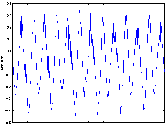
Analog signals are usually signals defined over continuous independent variable(s). Speech is produced by your vocal cords exciting acoustic resonances in your vocal tract. The result is pressure waves propagating in the air, and the speech signal thus corresponds to a function having independent variables of space and time and a value corresponding to air pressure: s(x, t) (Here we use vector notation x to denote spatial coordinates). When you record someone talking, you are evaluating the speech signal at a particular spatial location, x0 say. An example of the resulting waveform s(x0, t) is shown in this figure.
Photographs are static, and are continuous-valued signals defined over space. Black-and-white images have only one value at each point in space, which amounts to its optical reflection properties. In Figure 1.2, an image is shown, demonstrating that it (and all other images as well) are functions of two independent spatial variables.
 (a) | 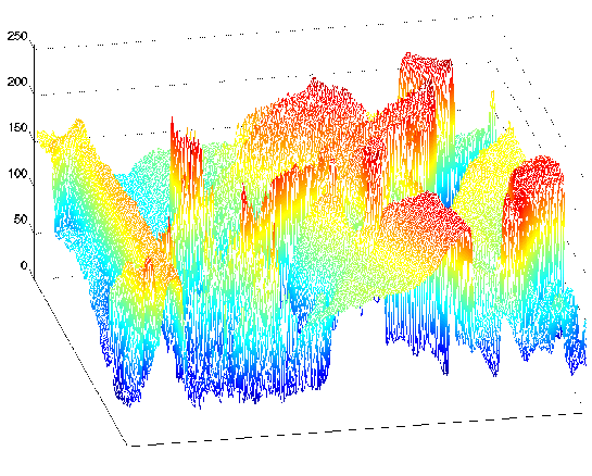 (b) |
Color images have values that express how reflectivity depends on the optical spectrum. Painters long ago found that mixing together combinations of the so-called primary colors--red, yellow and blue--can produce very realistic color images. Thus, images today are usually thought of as having three values at every point in space, but a different set of colors is used: How much of red, green and blue is present. Mathematically, color pictures are multivalued--vector-valued--signals: s(x)=(r(x), g(x), b(x))T.
Interesting cases abound where the analog signal depends not on a continuous variable, such as time, but on a discrete variable. For example, temperature readings taken every hour have continuous--analog--values, but the signal's independent variable is (essentially) the integers.
The word "digital" means discrete-valued and implies the signal has an integer-valued independent variable. Digital information includes numbers and symbols (characters typed on the keyboard, for example). Computers rely on the digital representation of information to manipulate and transform information. Symbols do not have a numeric value, and each is represented by a unique number. The ASCII character code has the upper- and lowercase characters, the numbers, punctuation marks, and various other symbols represented by a seven-bit integer. For example, the ASCII code represents the letter a as the number 97 and the letter A as 65 . Table 1.1 shows the international convention on associating characters with integers.
Signals are manipulated by systems. Mathematically, we represent what a system does by the notation y(t)=S(x(t)) , with x representing the input signal and y the output signal.
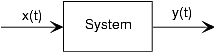
This notation mimics the mathematical symbology of a function: A system's input is analogous to an independent variable and its output the dependent variable. For the mathematically inclined, a system is a functional: a function of a function (signals are functions).
Simple systems can be connected together--one system's output becomes another's input--to accomplish some overall design. Interconnection topologies can be quite complicated, but usually consist of weaves of three basic interconnection forms.
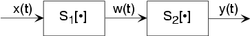
The simplest form is when one system's output is connected only to another's input. Mathematically, w(t)=S1(x(t)) , and y(t)=S2(w(t)) , with the information contained in x(t) processed by the first, then the second system. In some cases, the ordering of the systems matter, in others it does not. For example, in the fundamental model of communication the ordering most certainly matters.
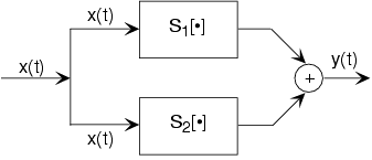
A signal x(t) is routed to two (or more) systems, with this signal appearing as the input to all systems simultaneously and with equal strength. Block diagrams have the convention that signals going to more than one system are not split into pieces along the way. Two or more systems operate on x(t) and their outputs are added together to create the output y(t) . Thus, y(t)=S1(x(t))+S2(x(t)) , and the information in x(t) is processed separately by both systems.
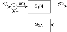
The subtlest interconnection configuration has a system's output also contributing to its input. Engineers would say the output is "fed back" to the input through system 2, hence the terminology. The mathematical statement of the feedback interconnection is that the feed-forward system produces the output: y(t)=S1(e(t)) . The input e(t) equals the input signal minus the output of some other system's output to y(t) : e(t)=x(t)−S2(y(t)) . Feedback systems are omnipresent in control problems, with the error signal used to adjust the output to achieve some condition defined by the input (controlling) signal. For example, in a car's cruise control system, x(t) is a constant representing what speed you want, and y(t) is the car's speed as measured by a speedometer. In this application, system 2 is the identity system (output equals input).
Mathematically, analog signals are functions having as their independent variables continuous quantities, such as space and time. Discrete-time signals are functions defined on the integers; they are sequences. As with analog signals, we seek ways of decomposing discrete-time signals into simpler components. Because this approach leading to a better understanding of signal structure, we can exploit that structure to represent information (create ways of representing information with signals) and to extract information (retrieve the information thus represented). For symbolic-valued signals, the approach is different: We develop a common representation of all symbolic-valued signals so that we can embody the information they contain in a unified way. From an information representation perspective, the most important issue becomes, for both real-valued and symbolic-valued signals, efficiency: what is the most parsimonious and compact way to represent information so that it can be extracted later.
A discrete-time signal is represented symbolically as s(n) , where n={…, -1, 0, 1, …} .
We usually draw discrete-time signals as stem plots to emphasize the fact they are functions defined only on the integers. We can delay a discrete-time signal by an integer just as with analog ones. A signal delayed by m samples has the expression s(n−m) .
The most important signal is, of course, the complex exponential sequence.
Note that the frequency variable f is dimensionless and that adding an integer to the frequency of the discrete-time complex exponential has no effect on the signal's value.

This derivation follows because the complex exponential evaluated at an integer multiple of 2π equals one. Thus, we need only consider frequency to have a value in some unit-length interval.
Discrete-time sinusoids have the obvious form
s(n)=Acos(2πfn+φ)
. As opposed to analog complex exponentials and
sinusoids that can have their frequencies be any real value,
frequencies of their discrete-time counterparts yield unique
waveforms only when
f
lies in the interval
 . This choice of frequency interval is arbitrary; we can also choose the frequency to lie in the interval
[0, 1)
.
How to choose a unit-length interval for a sinusoid's frequency will become evident later.
. This choice of frequency interval is arbitrary; we can also choose the frequency to lie in the interval
[0, 1)
.
How to choose a unit-length interval for a sinusoid's frequency will become evident later.
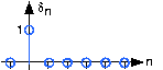
The second-most important discrete-time signal is the unit sample, which is defined to be

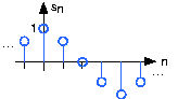
Examination of a discrete-time signal's plot, like that of the cosine signal shown in Figure 1.7, reveals that all signals consist of a sequence of delayed and scaled unit samples. Because the value of a sequence at each integer m is denoted by s(m) and the unit sample delayed to occur at m is written δ(n−m) , we can decompose any signal as a sum of unit samples delayed to the appropriate location and scaled by the signal value.

This kind of decomposition is unique to discrete-time signals, and will prove useful subsequently.
The unit sample in discrete-time is well-defined at the origin, as opposed to the situation with analog signals.

An interesting aspect of discrete-time signals is that the