This section introduces sampling. Sampling is the necessary fundament for all digital signal processing and communication. Sampling can be defined as the process of measuring an analog signal at distinct points.

Digital representation of analog signals offers advantages in terms of

Figure 2.1. 

Claude Elwood Shannon (1916-2001)

Claude Shannon has been called the father of information theory, mainly due to his landmark papers on the "Mathematical theory of communication". Harry Nyquist was the first to state the sampling theorem in 1928, but it was not proven until Shannon proved it 21 years later in the paper "Communications in the presence of noise".

In this chapter we will be using the following notation

Finished? Have at look at: Proof; Illustrations; Matlab Example; Aliasing applet; Hold operation; System view; Exercises

As mentioned earlier, sampling is the necessary fundament when we want to apply digital signal processing on analog signals.

Here we present the proof of the sampling theorem. The proof is divided in two. First we find an expression for the spectrum of the signal resulting from sampling the original signal x(t). Next we show that the signal x(t) can be recovered from the samples. Often it is easier using the frequency domain when carrying out a proof, and this is also the case here.

By sampling x(t) every T_s second we obtain x_s(n). The inverse fourier transform of this time discrete signal is

()

For convenience we express the equation in terms of the real angular frequency Ω using ω=ΩT_s. We then obtain

()

The inverse fourier transform of a continuous signal is

()

From this equation we find an expression for x (nT_s)

()

To account for the difference in region of integration we split the integration in Equation into subintervals of length and then take the sum over the resulting integrals to obtain the complete area.

()

Then we change the integration variable, setting

()

We obtain the final form by observing that ⅇ^ⅈ2πkn=1 , reinserting η=Ω and multiplying by

()

To make x_s(n)=x(nT_s) for all values of n, the integrands in Equation and Equation have to agreee, that is

()

This is a central result. We see that the digital spectrum consists of a sum of shifted versions of the original, analog spectrum. Observe the periodicity!

We can also express this relation in terms of the digital angular frequency ω=ΩT_s

()

This concludes the first part of the proof. Now we want to find a reconstruction formula, so that we can recover x(t) from x_s(n).

For a bandlimited signal the inverse fourier transform is

()

In the interval we are integrating we have: . Substituting this relation into Equation we get

()

Using the DTFT relation for X_s(ⅇ^ⅈΩT_s) we have

()

Interchanging integration and summation (under the assumption of convergence) leads to

()

Finally we perform the integration and arrive at the important reconstruction formula

()

(Thanks to R.Loos for pointing out an error in the proof.)

Go to Introduction; Illustrations; Matlab Example; Hold operation; Aliasing applet; System view; Exercises ?

We start off with an analog signal. This can for example be the sound coming from your stereo at home or your friend talking.

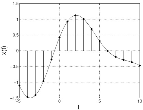
The signal is then sampled uniformly. Uniform sampling implies that we sample every T_s seconds. In Figure 2.2 we see an analog signal. The analog signal has been sampled at times t=nT_s.

Figure 2.2. 

Analog signal, samples are marked with dots.

In signal processing it is often more convenient and easier to work in the frequency domain. So let's look at at the signal in frequency domain, Figure 2.3. For illustration purposes we take the frequency content of the signal as a triangle. (If you Fourier transform the signal in Figure 2.2 you will not get such a nice triangle.)

Figure 2.3. 

The spectrum X(ⅈΩ) .

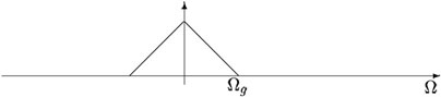
Notice that the signal in Figure 2.3 is bandlimited. We can see that the signal is bandlimited because X(ⅈΩ) is zero outside the interval [–Ω_g, Ω_g] . Equivalentely we can state that the signal has no angular frequencies above Ω_g, corresponding to no frequencies above .

Now let's take a look at the sampled signal in the frequency domain. While proving the sampling theorem we found the the spectrum of the sampled signal consists of a sum of shifted versions of the analog spectrum. Mathematically this is described by the following equation:

()