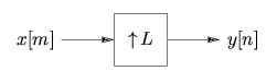
The operation of upsampling by factor L∈ℕ describes the insertion of L−1 zeros between every sample of the input signal. This is denoted by " ↑L " in block diagrams, as in Figure 4.1.
Formally, upsampling can be expressed in the time domain as
 In the z-domain,
 and substituting
z=ⅇⅈω
for the DTFT,
and substituting
z=ⅇⅈω
for the DTFT,
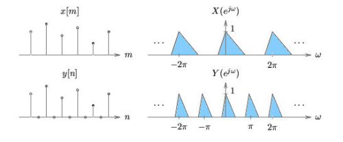
As shown in Figure 4.2, upsampling compresses the DTFT by a factor of L along with the ω axis.
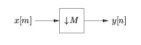
The operation of downsampling by factor M∈ℕ describes the process of keeping every Mth sample and discarding the rest. This is denoted by " ↓M " in block diagrams, as in Figure 4.3.
Formally, downsampling can be written as y[n]=x[nM] In the z domain,
where


Translating to the frequency domain,

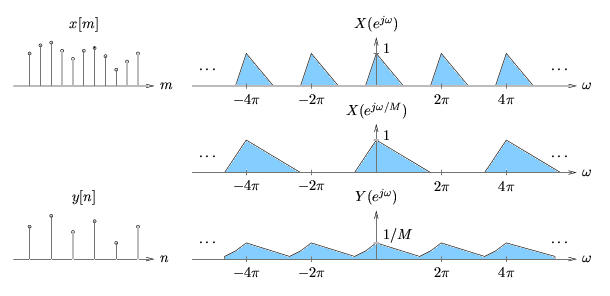
As shown in Figure 4.4, downsampling expands each
2π
-periodic repetition of
X(ⅇⅈω)
by a factor of M along the
ω axis, and reduces the gain
by a factor of M. If
x[m] is not bandlimited to
 ,
aliasing may result from spectral overlap.
,
aliasing may result from spectral overlap.
When performing a frequency-domain analysis of systems with up/downsamplers, it is strongly recommended to carry out the analysis in the z -domain until the last step, as done above. Working directly in the ⅇⅈω-domain can easily lead to errors.
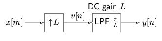
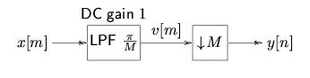
Interpolation is the process of upsampling and filtering a signal to increase its effective sampling rate. To be more specific, say that
x[m]
is an (unaliased) T-sampled version of
xc(t)
and
v[n]
is an L-upsampled version version of
x[m]
.
If we filter
v[n]
with an ideal -bandwidth lowpass filter (with DC gain L) to obtain
y[n]
, then
y[n]
will be a  -sampled version of
xc(t)
. This process is illustrated in Figure 4.5.
-sampled version of
xc(t)
. This process is illustrated in Figure 4.5.
We justify our claims about interpolation using frequency-domain arguments. From the sampling theorem, we know that T- sampling xc(t) to create x[n] yields

After upsampling by factor L,
Equation implies
 Lowpass filtering with cutoff
  and gain
L yields
and gain
L yields
 since the spectral copies with indices other than k=lL (for
l∈ℤ) are removed.
Clearly, this process yields a
since the spectral copies with indices other than k=lL (for
l∈ℤ) are removed.
Clearly, this process yields a  -shaped version of
xc(t)
.
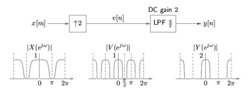
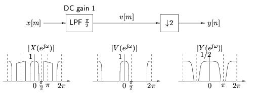
Figure 4.6 illustrates these frequency-domain arguments for
L=2.
-shaped version of
xc(t)
.
Figure 4.6 illustrates these frequency-domain arguments for
L=2.
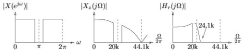
The digital audio signal on a CD is a 44.1kHz sampled representation of a continuous signal with bandwidth 20kHz . With a standard ZOH-DAC, the analog reconstruction filter would have passband edge at 20kHz and stopband edge at 24.1kHz . (See Figure 4.7) With such a narrow transition band, this would be a difficult (and expensive) filter to build.
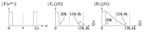
If digital interpolation is used prior to reconstruction, the effective sampling rate can be increased and the reconstruction filter's transition band can be made much wider, resulting in a much simpler (and cheaper) analog filter. Figure 4.8 illustrates the case of interpolation by 4. The reconstruction filter has passband edge at 20kHz and stopband edge at 156.4kHz , resulting in a much wider transition band and therefore an easier filter design.
Decimation is the process of filtering and downsampling a signal to decrease its effective sampling rate, as illustrated in Figure 4.9. The filtering is employed to prevent aliasing that might otherwise result from downsampling.
To be more specific, say that
xc(t)=xl(t)+xb(t)
where
xl(t)
is a lowpass component bandlimited to
 Hz and
xb(t)
is a bandpass component with energy between
Hz and
xb(t)
is a bandpass component with energy between
 and
.
If sampling
xc(t)
with interval T
yields an unaliased discrete representation
x[m], then decimating
x[m] by a factor
M will yield
y[n], an unaliased
MT-sampled
representation of lowpass component
xl(t)
.
and
.
If sampling
xc(t)
with interval T
yields an unaliased discrete representation
x[m], then decimating
x[m] by a factor
M will yield
y[n], an unaliased
MT-sampled
representation of lowpass component
xl(t)
.
We offer the following justification of the previously described
decimation procedure. From the sampling theorem, we have

The bandpass component
Xb(ⅈΩ)
is the removed by
-lowpass
filtering, giving
 Finally, downsampling yields
which is clearly a MT-sampled version of xl(t) . A frequency-domain illustration for M=2 appears in Figure 4.10.
Interpolation by L and decimation
by M can be combined to change the
effective sampling rate of a signal by the rational factor
. This process is called resampling or
sample-rate conversion. Rather than cascading an
anti-imaging filter for interpolation with an anti-aliasing
filter for decimation, we implement one filter with the minimum
of the two cutoffs
and the multiplication of the two DC gains
(L and
1), as illustrated in Figure 4.11.

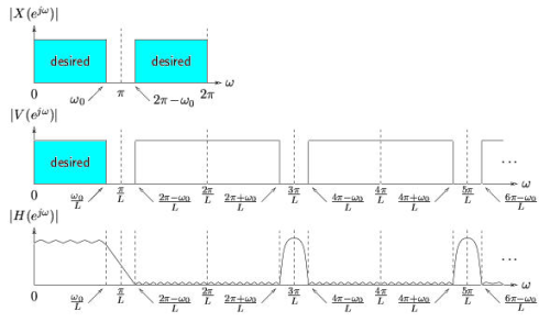
First we treat filter design for interpolation.
Consider an input signal
x[n]
that is
ω0-bandlimited in the DTFT domain.
If we upsample by factor
L to get
v[m]
, the desired portion of
V(ⅇⅈω)
is the spectrum in
,
while the undesired portion is the remainder of
[–π, π)
.
Noting from Figure 4.12 that
V(ⅇⅈω)
has zero energy in the regions
the anti-imaging filter can be designed with transition bands in these regions (rather than passbands or stopbands). For a given number of taps, the additional degrees of freedom offered by these transition bands allows for better responses in the passbands and stopbands. The resulting filter design specifications are shown in the bottom subplot below.
Next we treat filter design for decimation. Say that the
desired spectral component of the input
signal is bandlimited to
 and we have decided to downsample by M.
The goal is to minimally distort the input spectrum over
, i.e., the post-decimation
spectrum over
[–ω0, ω0)
and we have decided to downsample by M.
The goal is to minimally distort the input spectrum over
, i.e., the post-decimation
spectrum over
[–ω0, ω0)