Before now, you have probably dealt strictly with the theory behind signals and systems, as well as look at some the basic characteristics of signals and systems. In doing so you have developed an important foundation; however, most electrical engineers do not get to work in this type of fantasy world. In many cases the signals of interest are very complex due to the randomness of the world around them, which leaves them noisy and often corrupted. This often causes the information contained in the signal to be hidden and distorted. For this reason, it is important to understand these random signals and how to recover the necessary information.
For this study of signals and systems, we will divide signals into two groups: those that have a fixed behavior and those that change randomly. As most of you have probably already dealt with the first type, we will focus on introducing you to random signals. Also, note that we will be dealing strictly with discrete-time signals since they are the signals we deal with in DSP and most real-world computations, but these same ideas apply to continuous-time signals.
Most introductions to signals and systems deal strictly with deterministic signals. Each value of these signals are fixed and can be determined by a mathematical expression, rule, or table. Because of this, future values of any deterministic signal can be calculated from past values. For this reason, these signals are relatively easy to analyze as they do not change, and we can make accurate assumptions about their past and future behavior.
Unlike deterministic signals, stochastic signals, or random signals, are not so nice. Random signals cannot be characterized by a simple, well-defined mathematical equation and their future values cannot be predicted. Rather, we must use probability and statistics to analyze their behavior. Also, because of their randomness, average values from a collection of signals are usually studied rather than analyzing one individual signal.
As mentioned above, in order to study random signals, we want to look at a collection of these signals rather than just one instance of that signal. This collection of signals is called a random process.
A family or ensemble of signals that correspond to every possible outcome of a certain signal measurement. Each signal in this collection is referred to as a realization or sample function of the process.
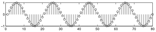
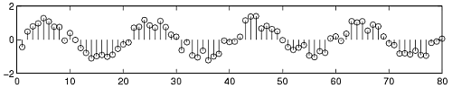
As an example of a random process, let us look at the Random Sinusoidal Process below. We use f[n]=Asin(ωn+φ) to represent the sinusoid with a given amplitude and phase. Note that the phase and amplitude of each sinusoid is based on a random number, thus making this a random process.
A random process is usually denoted by X(t) or X[n] , with x(t) or x[n] used to represent an individual signal or waveform from this process.
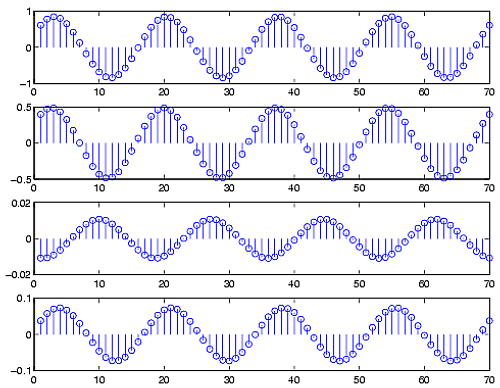
In many notes and books, you might see the following notation and terms used to describe different types of random processes. For a discrete random process, sometimes just called a random sequence, t represents time that has a finite number of values. If t can take on any value of time, we have a continuous random process. Often times discrete and continuous refer to the amplitude of the process, and process or sequence refer to the nature of the time variable. For this study, we often just use random process to refer to a general collection of discrete-time signals, as seen above in Figure 5.3.
From the definition of a random process, we know that all random processes are composed of random variables, each at its own unique point in time. Because of this, random processes have all the properties of random variables, such as mean, correlation, variances, etc.. When dealing with groups of signals or sequences it will be important for us to be able to show whether of not these statistical properties hold true for the entire random process. To do this, the concept of stationary processes has been developed. The general definition of a stationary process is:
a random process where all of its statistical properties do not vary with time
Processes whose statistical properties do change are referred to as nonstationary.
Understanding the basic idea of stationarity will help you to be able to follow the more concrete and mathematical definition to follow. Also, we will look at various levels of stationarity used to describe the various types of stationarity characteristics a random process can have.
In order to properly define what it means to be stationary from a mathematical standpoint, one needs to be somewhat familiar with the concepts of distribution and density functions. If you can remember your statistics then feel free to skip this section!
Recall that when dealing with a single random variable, the probability distribution function is a simply tool used to identify the probability that our observed random variable will be less than or equal to a given number. More precisely, let X be our random variable, and let x be our given value; from this we can define the distribution function as
This same idea can be applied to instances where we have multiple random variables as well. There may be situations where we want to look at the probability of event X and Y both occurring. For example, below is an example of a second-order joint distribution function.
While the distribution function provides us with a full view of our variable or processes probability, it is not always the most useful for calculations. Often times we will want to look at its derivative, the probability density function (pdf). We define the the pdf as

Equation reveals some of the physical significance of the density function. This equations tells us the probability that our random variable falls within a given interval can be approximated by fx(x)dx . From the pdf, we can now use our knowledge of integrals to evaluate probabilities from the above approximation. Again we can also define a joint density function which will include multiple random variables just as was done for the distribution function. The density function is used for a variety of calculations, such as finding the expected value or proving a random variable is stationary, to name a few.
The above examples explain the distribution and density functions in terms of a single random variable, X. When we are dealing with signals and random processes, remember that we will have a set of random variables where a different random variable will occur at each time instance of the random process, X(tk) . In other words, the distribution and density function will also need to take into account the choice of time.
Below we will now look at a more in depth and mathematical definition of a stationary process. As was mentioned previously, various levels of stationarity exist and we will look at the most common types.
A random process is classified as first-order stationary if its first-order probability density function remains equal regardless of any shift in time to its time origin. If we let xt1 represent a given value at time t1, then we define a first-order stationary as one that satisfies the following equation:
The physical significance of this equation is that our density function, fx(xt1) , is completely independent of t1 and thus any time shift, τ.
The most important result of this statement, and the identifying characteristic of any first-order stationary process, is the fact that the mean is a constant, independent of any time shift. Below we show the results for a random process, X, that is a discrete-time signal, x[n] .

A random process is classified as second-order stationary if its second-order probability density function does not vary over any time shift applied to both values. In other words, for values xt1 and xt2 then we will have the following be equal for an arbitrary time shift τ.
From this equation we see that the absolute time does not affect our functions, rather it only really depends on the time difference between the two variables. Looked at another way, this equation can be described as
These random processes are often referred to as strict sense stationary (SSS) when all of the distribution functions of the process are unchanged regardless of the time shift applied to them.
For a second-order stationary process, we need to look at the autocorrelation function to see its most important property. Since we have already stated that a second-order stationary process depends only on the time difference, then all of these types of processes have the following property:

As you begin to work with random processes, it will become evident that the strict requirements of a SSS process is more than is often necessary in order to adequately approximate our calculations on random processes. We define a final type of stationarity, referred to as wide-sense stationary (WSS), to have slightly more relaxed requirements but ones that are still enough to provide us with adequate results. In order to be WSS a random process only needs to meet the following two requirements.

E[X(t+τ)]=Rxx(τ)
Note that a second-order (or SSS) stationary process will always be WSS; however, the reverse will not always hold true.
In order to study the characteristics of a random process, let us look at some of the basic properties and operations of a random process. Below we will focus on the operations of the random signals that compose our random processes. We will denote our random process with X and a random variable from a random process or signal by x.
Finding the average value of a set of random signals or random variables is probably the most fundamental concepts we use in evaluating random processes through any sort of statistical method. The mean of a random process is the average of all realizations of that process. In order to find this average, we must look at a random signal over a range of time (possible values) and determine our average from this set of values. The mean, or average, of a random process, x(t) , is given by the following equation:

This equation may seem quite cluttered at first glance, but we want to introduce you to the various notations used to represent the mean of a random signal or process. Throughout texts and other readings, remember that these will all equal the same thing. The symbol, μx(t) , and the X with a bar over it are often used as a short-hand to represent an average, so you might see it in certain textbooks. The other important notation used is, E[X] , which represents the "expected value of X" or the mathematical expectation. This notation is very common and will appear again.
If the random variables, which make up our random process, are discrete or quantized values, such as in a binary process, then the integrals become summations over all the possible values of the random variable. In this case, our expected value becomes

If we have two random signals or variables, their averages can reveal how the two signals interact. If the product of the two individual averages of both signals do not equal the average of the product of the two signals, then the two signals are said to be linearly independent, also referred to as uncorrelated.
In the case where we have a random process in which only one sample can be viewed at a time, then we will often not have all the information available to calculate the mean using the density function as shown above. In this case we must estimate the mean through the time-av