Questions or comments concerning this laboratory should be directed to Prof. Charles A. Bouman, School of Electrical and Computer Engineering, Purdue University, West Lafayette IN 47907; (765) 494-0340; bouman@ecn.purdue.edu
This is the first part of a two week laboratory in digital filter design. The first week of the laboratory covers some basic examples of FIR and IIR filters, and then introduces the concepts of FIR filter design. Then the second week covers systematic methods of designing both FIR and IIR filters.
In digital signal processing applications, it is often necessary to change the relative amplitudes of frequency components or remove undesired frequencies of a signal. This process is called filtering. Digital filters are used in a variety of applications. In Laboratory 4, we saw that digital filters may be used in systems that perform interpolation and decimation on discrete-time signals. Digital filters are also used in audio systems that allow the listener to adjust the bass (low-frequency energy) and the treble (high frequency energy) of audio signals.
Digital filter design requires the use of both frequency domain and time domain techniques. This is because filter design specifications are often given in the frequency domain, but filters are usually implemented in the time domain with a difference equation. Typically, frequency domain analysis is done using the Z-transform and the discrete-time Fourier Transform (DTFT).
In general, a linear and time-invariant causal digital filter with input x(n) and output y(n) may be specified by its difference equation

where bi and ak are coefficients which parameterize the filter. This filter is said to have N zeros and M poles. Each new value of the output signal, y(n), is determined by past values of the output, and by present and past values of the input. The impulse response, h(n), is the response of the filter to an input of δ(n), and is therefore the solution to the recursive difference equation

There are two general classes of digital filters: infinite impulse response (IIR) and finite impulse response (FIR). The FIR case occurs when ak=0, for all k. Such a filter is said to have no poles, only zeros. In this case, the difference equation in Equation 6.2 becomes

Since Equation 6.3 is no longer recursive, the impulse response has finite duration N.
In the case where ak≠0, the difference equation usually represents an IIR filter. In this case, Equation 6.2 will usually generate an impulse response which has non-zero values as n→∞. However, later we will see that for certain values of ak≠0 and bi, it is possible to generate an FIR filter response.
The Z-transform is the major tool used for analyzing the frequency response of filters and their difference equations. The Z-transform of a discrete-time signal, x(n), is given by

where z is a complex variable. The DTFT may be thought of as a special case of the Z-transform where z is evaluated on the unit circle in the complex plane.

From the definition of the Z-transform, a change of variable m=n–K shows that a delay of K samples in the time domain is equivalent to multiplication by z–K in the Z-transform domain.

We may use this fact to re-write Equation 6.1 in the Z-transform domain, by taking Z-transforms of both sides of the equation:

From this formula, we see that any filter which can be represented by a linear difference equation with constant coefficients has a rational transfer function (i.e. a transfer function which is a ratio of polynomials). From this result, we may compute the frequency response of the filter by evaluating H(z) on the unit circle:

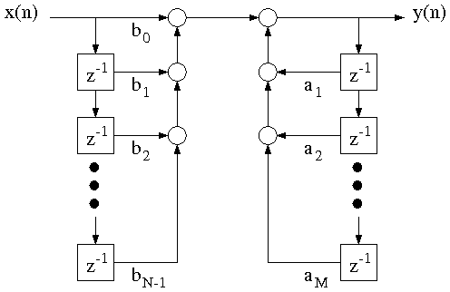
There are many different methods for implementing a general recursive difference equation of the form Equation 6.1. Depending on the application, some methods may be more robust to quantization error, require fewer multiplies or adds, or require less memory. Figure 6.1 shows a system diagram known as the direct form implementation; it works for any discrete-time filter described by the difference equation in Equation 6.1. Note that the boxes containing the symbol z–1 represent unit delays, while a parameter written next to a signal path represents multiplication by that parameter.
Download the files, nspeech1.mat and DTFT.m for the following section.
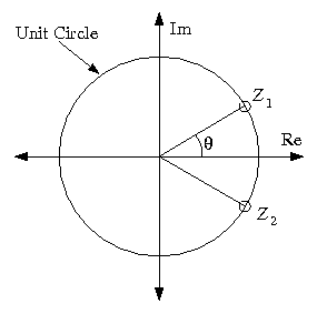
To illustrate the use of zeros in filter design, you will design a simple second order FIR filter with the two zeros on the unit circle as shown in Figure 6.2. In order for the filter's impulse response to be real-valued, the two zeros must be complex conjugates of one another:
where θ is the angle of z1 relative to the positive real axis. We will see later that θ∈[0,π] may be interpreted as the location of the zeros in the frequency response.
The transfer function for this filter is given by

Use this transfer function to determine the difference equation for this filter. Then draw the corresponding system diagram and compute the filter's impulse response h(n).
This filter is an FIR filter
because it has impulse response h(n) of finite duration.
Any filter with only zeros and no poles other than those
at 0 and ±∞ is an FIR filter.
Zeros in the transfer function represent frequencies that are
not passed through the filter.
This can be useful for removing unwanted frequencies in a signal.
The fact that Hf(z) has zeros at e±jθ implies that
 . This means that
the filter will not pass pure sine waves at a frequency
of ω=θ.
. This means that
the filter will not pass pure sine waves at a frequency
of ω=θ.
Use Matlab to compute and plot the magnitude of the filter's
frequency response  as a function of
ω on the interval –π<ω<π, for
the following three values of θ:
as a function of
ω on the interval –π<ω<π, for
the following three values of θ:
| i):
(6.12)
θ
=
π
/
6
|
| ii):
(6.13)
θ
=
π
/
3
|
| ii):
(6.14)
θ
=
π
/
2
|
Put all three plots on the same figure using the
subplot command.
Submit the difference equation, system diagram, and the analytical expression of the impulse response for the filter Hf(z). Also submit the plot of the magnitude response for the three values of θ. Explain how the value of θ affects the magnitude of the filter's frequency response.
In the next experiment, we will use the filter Hf(z)
to remove an undesirable sinusoidal interference from
a speech signal.
To run the experiment, first download the audio signal
nspeech1.mat, and the
M-file
DTFT.m
Load nspeech1.mat into Matlab using the command load nspeech1.
This will load the signal nspeech1 into the workspace.
Play nspeech1 using the sound command,
and then plot 101 samples of the signal for the time indices (100:200).
We will next use the DTFT command to compute samples of the
DTFT of the audio signal.
The DTFT command has the syntax
[X,w]=DTFT(x,M)
where x
is a signal which is assumed to start at time n=0,
and M specifies the number of output points of the DTFT.
The command [X,w]=DTFT(x,0)
will generate a DTFT that
is the same duration as the input; if this
is not sufficient, it may be increased by specifying M
.
The outputs of the function are a vector X
containing the
samples of the DTFT, and a vector w
containing
the corresponding frequencies of these samples.
Compute the magnitude of the DTFT of 1001 samples
of the audio signal for the time indices (100:1100).
Plot the magnitude of the DTFT samples versus frequency
for |ω|<π.
Notice that there are two large peaks corresponding to the sinusoidal
interference signal.
Use the Matlab max command to determine the
exact frequency of the peaks.
This will be the value of θ that we will use for filtering
with Hf(z).
Use the command [Xmax,Imax]=max(abs(X))
to find
the value and index of the maximum element in X
.
θ can be derived using this index.
Write a Matlab function FIRfilter(x)
that implements the filter Hf(z)
with the measured value of θ
and outputs the filtered signal (Hint:
Use convolution).
Apply the new function FIRfilter to the nspeech1 vector
to attenuate the sinusoidal interference.
Listen to the filtered signal to hear the effects of the filter.
Plot 101 samples of the signal for the time indices (100:200),
and plot the magnitude of the DTFT of 1001 samples
of the filtered signal for the time indices (100:1100).
For both the original audio signal and the filtered output, hand in the following:
The time domain plot of 101 samples.
The plot of the magnitude of the DTFT for 1001 samples.
Also hand in the code for the FIRfilter filtering function.
Comment on how the frequency content of the signal changed
after filtering.
Is the filter we used a lowpass, highpass, bandpass, or a
bandstop filter?
Comment on how the filtering changed the
quality of the audio signal.
Download the file pcm.mat for the following section.
While zeros attenuate a filtered signal, poles amplify signals that are near their frequency. In this section, we will illustrate how poles can be used to separate a narrow-band signal from adjacent noise. Such filters are commonly used to separate modulated signals from background noise in applications such as radio-frequency demodulation.
Consider the following transfer function for a second order IIR filter with complex-conjugate poles:

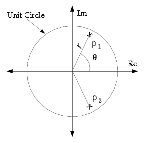
Figure 6.3 shows the locations of the two poles of this filter. The poles have the form

where r is the distance from the origin, and θ is the angle of p1 relative to the positive real axis. From the theory of Z-transforms, we know that a causal filter is stable if and only if its poles are located within the unit circle. This implies that this filter is stable if and only if |r|<1. However, we will see that by locating the poles close to the unit circle, the filter's bandwidth may be made extremely narrow around θ.
This two-pole system is an example of an IIR filter because its impulse response has infinite duration. Any filter with nontrivial poles (not at z = 0 or ±∞) is an IIR filter unless the poles are canceled by zeros.
Calculate the magnitude of the filter's frequency response  on |ω|<π for θ=π/3 and the following three values of r.
Put all three plots on the same figure using the subplot command.
Submit the difference equation, system diagram and the analytical expression of the impulse response for Hi(z). Also submit the plot of the magnitude of the frequency response for each value of r. Explain how the value of r affects this magnitude.
In the following experiment,
we will use the filter Hi(z) to separate a modulated sinusoid
from background noise.
To run the experiment,
first download the file
pcm.mat
and load it into the Matlab
workspace using the command load pcm
.
Play pcm using the sound command.
Plot 101 samples of the signal for indices (100:200),
and then compute the magnitude of the DTFT of 1001 samples
of pcm using the time indices (100:1100).
Plot the magnitude of the DTFT samples versus radial frequency
for |ω|<π. The two peaks in the spectrum correspond
to the center frequency of the modulated signal.
The low amplitude wideband content is the background noise.
In this exercise, you will use the IIR filter described above to
amplify the desired signal, relative to the background noise.
The pcm signal is modulated at 3146Hz and sampled at 8kHz. Use these values to calculate the value of θ for the filter Hi(z). Remember from the sampling theorem that a radial frequency of 2π corresponds to the sampling frequency.
Write a Matlab function IIRfilter(x)
that implements the filter
Hi(z).
In this case, you need to use a for loop to implement the
recursive difference equation. Use your calculated value of θ
and r=0.995.
You can assume that y(n)
is equal to 0
for negative values of n.
Apply the new command IIRfilter