Questions or comments concerning this laboratory should be directed to Prof. Charles A. Bouman, School of Electrical and Computer Engineering, Purdue University, West Lafayette IN 47907; (765) 494-0340; bouman@ecn.purdue.edu
This is the second part of a two week laboratory in digital filter design. The first week of the laboratory covered some basic examples of FIR and IIR filters, and then introduced the concepts of filter design. In this week we will cover more systematic methods of designing both FIR and IIR filters.
Download DTFT.m for the following section.
We can generalize the idea of truncation by using different windowing functions to truncate an ideal filter's impulse response. Note that by simply truncating the ideal filter's impulse response, we are actually multiplying (or “windowing”) the impulse response by a shifted rect() function. This particular type of window is called a rectangular window. In general, the impulse reponse h(n) of the designed filter is related to the impulse response hideal(n) of the ideal filter by the relation
where w(n) is an N-point window. We assume that

where ωc is the cutoff frequency and N is the desired window length.
The rectangular window is defined as

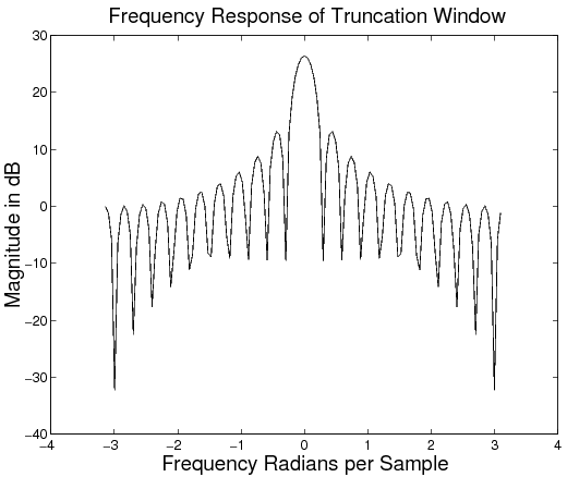
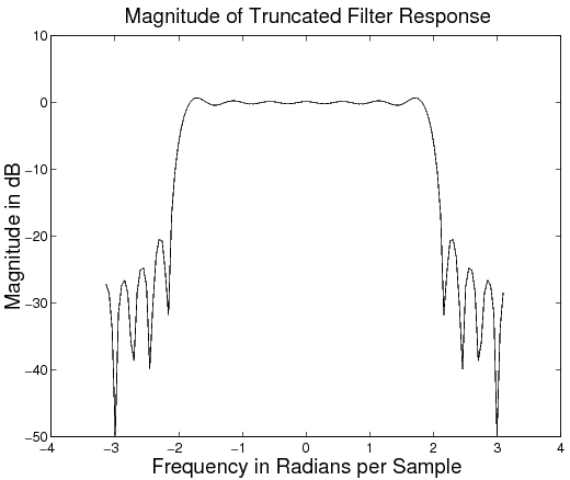
The DTFT of w(n) for N=21 is shown in Figure 7.1. The rectangular window is usually not preferred because it leads to the large stopband and passband ripple as shown in Figure 7.2.
More desirable frequency characteristics can be obtained by making a better selection for the window, w(n). In fact, a variety of raised cosine windows are widely used for this purpose. Some popular windows are listed below.
Hanning window (as defined in Matlab, command hann(N)):

Hamming window

Blackman window

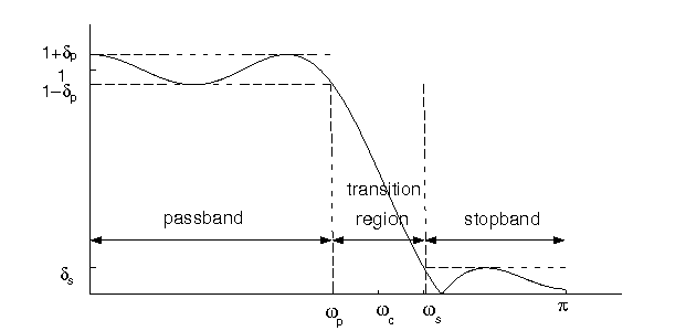
In filter design using different truncation windows, there are two key frequency domain effects that are important to the design: the transition band roll-off, and the passband and stopband ripple (see Figure 7.3 below). There are two corresponding parameters in the spectrum of each type of window that influence these filter parameters. The filter's roll-off is related to the width of center lobe of the window's magnitude spectrum. The ripple is influenced by the ratio of the mainlobe amplitude to the first sidelobe amplitude (or difference if using a dB scale). These two window spectrum parameters are not independent, and you should see a trend as you examine the spectra for different windows. The theoretical values for the mainlobe width and the peak-to-sidelobe amplitude are shown in Table 7.1.
| Window (length N) | Mainlobe width | Peak-to-sidelobe amplitude (dB) |
| Rectangular | 4 π / N | – 13 d B |
| Hanning | 8 π / N | – 32 d B |
| Hamming | 8 π / N | – 43 d B |
| Blackman | 12 π / N | – 58 d B |
Plot the rectangular, Hamming, Hanning, and Blackman window functions
of length 21 on a single figure using the subplot command.
You may use the Matlab commands hamming,
hann, and blackman.
Then compute and plot the DTFT magnitude of each of the four windows.
Plot the magnitudes on a decibel scale
(i.e., plot  ). Download and use the function
DTFT.m
to compute the DTFT.
). Download and use the function
DTFT.m
to compute the DTFT.
Use at least 512 sample points in computing the DTFT by
typing the command DTFT(window,512). Type help DTFT for
further information on this function.
Measure the null-to-null mainlobe width (in rad/sample)
and the peak-to-sidelobe amplitude (in dB)
from the logarithmic magnitude response plot
for each window type. The Matlab command zoom is helpful for this.
Make a table with these values and
the theoretical ones.
Now use a Hamming window to design a lowpass filter h(n) with a cutoff frequency of ωc=2.0 and length 21. Note: You need to use Equation 7.1 and Equation 7.2 for this design. In the same figure, plot the filter's impulse response, and the magnitude of the filter's DTFT in decibels.
Submit the figure containing the time domain plots of the four windows.
Submit the figure containing the DTFT (in decibels) of the four windows.
Submit the table of the measured and theoretical window spectrum parameters. Comment on how close the experimental results matched the ideal values. Also comment on the relation between the width of the mainlobe and the peak-to-sidelobe amplitude.
Submit the plots of your designed filter's impulse response and the magnitude of the filter's DTFT.
Download nspeech2.mat for the following section.
The standard windows of the "Filter Design Using Standard Windows" section are an improvement over simple truncation, but these windows still do not allow for arbitrary choices of transition bandwidth and ripple. In 1964, James Kaiser derived a family of near-optimal windows that can be used to design filters which meet or exceed any filter specification. The Kaiser window depends on two parameters: the window length N, and a parameter β which controls the shape of the window. Large values of β reduce the window sidelobes and therefore result in reduced passband and stopband ripple. The only restriction in the Kaiser filter design method is that the passband and stopband ripple must be equal in magnitude. Therefore, the Kaiser filter must be designed to meet the smaller of the two ripple constraints:

The Kaiser window function of length N is given by

where I0(·) is the zero'th order modified Bessel function of the first kind, N is the length of the window, and β is the shape parameter.
Kaiser found that values of β and N
could be chosen to meet any set of design parameters,
 , by defining
A=–20log10δ and using the following two equations:
, by defining
A=–20log10δ and using the following two equations:


where ⌈·⌉ is the ceiling function, i.e. ⌈x⌉ is the smallest integer which is greater than or equal to x.
To further investigate the Kaiser window, plot the Kaiser windows and their DTFT magnitudes (in dB) for N=21 and the following values of β:
For each case use at least 512 points in the plot of the DTFT.
To create the
Kaiser windows, use the Matlab command
kaiser(N,beta)
command where N
is the length of the filter and beta
is the shape parameter β.
To insure at least 512 points in the plot use the command
DTFT(window,512)
when computing the DTFT.
Submit the plots of the 3 Kaiser windows and the magnitude of their DTFT's in decibels. Comment on how the value β affects the shape of the window and the sidelobes of the DTFT.
Next use a Kaiser window to design a low pass filter, h(n), to remove the noise from the signal in nspeech2.mat using equations Equation 7.1 and Equation 7.2. To do this, use equations Equation 7.9 and Equation 7.10 to compute the values of β and N that will yield the following design specifications:

The low pass filter designed with the Kaiser method will automatically have a cut-off frequency centered between ωp and ωs.

Plot the magnitude of the DTFT of h(n) for |ω|<π . Create three plots in the same figure: one that shows the entire frequency response, and ones that zoom in on the passband and stopband ripple, respectively. Mark ωp, ωs, δp, and δs on these plots where appropriate. Note: Since the ripple is measured on a magnitude scale, DO NOT use a decibel scale on this set of plots.
From the Matlab prompt, compute the stopband and passband ripple (do not do this graphically). Record the stopband and passband ripple to three decimal places.
To compute the passband ripple, find the value of the DTFT at frequencies corresponding
to the passband using the command H(abs(w)<=1.8)
where H is the DTFT of h(n) and w is the corresponding vector
of frequencies. Then use this vector to compute the passband ripple.
Use a similar procedure for the stopband ripple.
Filter the noisy speech signal in
nspeech2.mat
using the filter you have designed.
Then compute the
DTFT of 400 samples of the filtered signal starting
at time n=20000 (i.e. 20001:20400
).
Plot the magnitude of the DTFT samples in decibels
versus frequency in radians for |ω|<π.
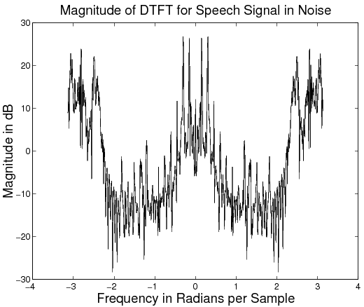
Compare this with the spectrum of the noisy speech signal shown
in Figure 7.4.
Play the noisy and filtered speech signals back using
sound and listen to them carefully.
Do the following:
Submit the values of β and N that you computed.
Submit the three plots of the filter's magnitude response. Make sure the plots are labeled.
Submit the values of the passband and stopband ripple. Does this filter meet the design specifications?
Submit the magnitude plot of the DTFT in dB for the filtered signal. Compare this plot to the plot of Figure 7.4.
Comment on how the frequency content and the audio quality of the filtered signal have changed after filtering.
Click here for help
on the firpm function for Parks-McClellan filter design.
Download the data file nspeech2.mat for the following section.
Kaiser windows are versatile since they allow the design of arbitrary filters which meet specific design constraints. However, filters designed with Kaiser windows still have a number of disadvantages. For example,
Kaiser filters are not guaranteed to be the minimum length filter which meets the design constraints.
Kaiser filters do not allow passband and stopband ripple to be varied independently.
Minimizing filter length is important because in many applications the length of the filter determines the amount of computation. For example, an FIR filter of length N may be directly implemented in the time domain by evaluating the expression