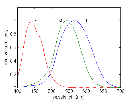
Color is a perceptual phenomenon related to the human response to different wavelengths of light, mainly in the region of 400 to 700 nanometers (nm). The perception of color arises from the sensitivities of three types of neurochemical sensors in the retina, known as the long (L), medium (M), and short (S) cones. The response of these sensors to photons is shown in Figure 17.1. Note that each sensor responds to a range of wavelengths.

Figure 17.1. 

Relative photon sensitivity of long (L), medium (M), and short (S) cones.

Due to this property of the human visual system, all colors can be modeled as combinations of the three primary color components: red (R), green (G), and blue (B). For the purpose of standardization, the CIE (Commission International de l'Eclairage — the International Commission on Illumination) designated the following wavelength values for the three primary colors: blue = 435.8nm, green = 546.1nm, and red = 700nm.

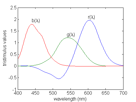
The relative amounts of the three primary colors of light required to produce a color of a given wavelength are called tristimulus values. Figure 17.2 shows the plot of tristimulus values using the CIE primary colors. Notice that some of the tristimulus values are negative, which indicates that colors at those wavelengths cannot be reproduced by the CIE primary colors.

Figure 17.2. 

Plot of tristimulus values using CIE primary colors.

A color space allows us to represent all the colors perceived by human beings. We previously noted that weighted combinations of stimuli at three wavelengths are sufficient to describe all the colors we perceive. These wavelengths form a natural basis, or coordinate system, from which the color measurement process can be described. In this lab, we will examine two common color spaces: RGB and YC_bC_r. For more information, refer to 1.

In YC_bC_r, the luminance parameter is related to an overall intensity of the image. The chrominance components are a measure of the relative intensities of the blue and red components. The inverse of the transformation in Equation 17.1 can easily be shown to be the following.

(17.2)

Download the files girl.tif and ycbcr.mat. For help on image command select the link.

You will be displaying both color and monochrome images in the following exercises. Matlab's image command can be used for both image types, but care must be taken for the command to work properly. Please see the help on the image command for details.

Download the RGB color image file girl.tif , and load it into Matlab using the imread command. Check the size of the Matlab array for this image by typing whos. Notice that this is a three dimensional array of type uint8. It contains three gray scale image planes corresponding to the red, green, and blue components for each pixel. Since each color pixel is represented by three bytes, this is commonly known as a 24-bit image. Display the color image using

image(A);

axis('image');

where A is the 3-D RGB array.

You can extract each of the color components using the following commands.

RGB = imread('girl.tif'); % color image is loaded into matrix RGB

R = RGB(:,:,1); % extract red component from RGB

G = RGB(:,:,2); % extract green component from RGB

B = RGB(:,:,3); % extract blue component from RGB

Use the subplot and image commands to plot the original image, along with each of the three color components. Note that while the original is a color image, each color component separately is a monochrome image. Use the syntax subplot(2,2,n) , where n=1,2,3,4, to place the four images in the same figure. Place a title on each of the images, and print the figure (use a color printer).

We will now examine the YC_bC_r color space representation. Download the file ycbcr.mat , and load it into Matlab using load ycbcr. This file contains a Matlab array for a color image in YC_bC_r format. The array contains three gray scale image planes that correspond to the luminance (Y) and two chrominance (C_bC_r) components. Use subplot(3,1,n) and image to display each of the components in the same figure. Place a title on each of the three monochrome images, and print the figure.

In order to properly display this color image, we need to convert it to RGB format. Write a Matlab function that will perform the transformation of Equation 17.2. It should accept a 3-D YC_bC_r image array as input, and return a 3-D RGB image array.

Now, convert the ycbcr array to an RGB representation and display the color image. Remember to convert the result to type uint8 before using the image command.

An interesting property of the human visual system, with respect to the YC_bC_r color space, is that we are much more sensitive to distortion in the luminance component than in the chrominance components. To illustrate this, we will smooth each of these components with a Gaussian filter and view the results.

You may have noticed when you loaded ycbcr.mat into Matlab that you also loaded a 5×5 matrix, h. This is a 5×5 Gaussian filter with σ²=2.0. (See the first week of the experiment for more details on this type of filter.) Alter the ycbcr array by filtering only the luminance component, ycbcr(:,:,1) , using the Gaussian filter (use the filter2 function). Convert the result to RGB, and display it using image. Now alter ycbcr by filtering both chrominance components, ycbcr(:,:,2) and ycbcr(:,:,3), using the Gaussian filter. Convert this result to RGB, and display it using image.

Use subplot(3,1,n) to place the original and two filtered versions of the ycbcr image in the same figure. Place a title on each of the images, and print the figure (in color). Do you see a significant difference between the filtered versions and the original image? This is the reason that YC_bC_r is often used for digital video. Since we are not very sensitive to corruption of the chrominance components, we can afford to lose some information in the encoding process.

As was discussed in the first week of this lab, an 8-bit monochrome image allows 256 distinct gray levels. Such images can be displayed on a computer monitor if the hardware supports the required number intensity levels. However, some output devices print or display images with much fewer gray levels. In the extreme case, the gray scale images must be converted to binary images, where pixels can only be black or white.

The simplest way of converting to a binary image is based on thresholding, i.e. two-level (one-bit) quantization. Let f(i,j) be a gray scale image, and b(i,j) be the corresponding binary image based on thresholding. For a given threshold T, the binary image is computed as the following:

(17.3)

(a)

(b)

Figure 17.3. 

(1) Original gray scale image. (2) Binary image produced by simple fixed thresholding.

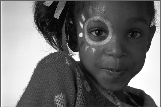
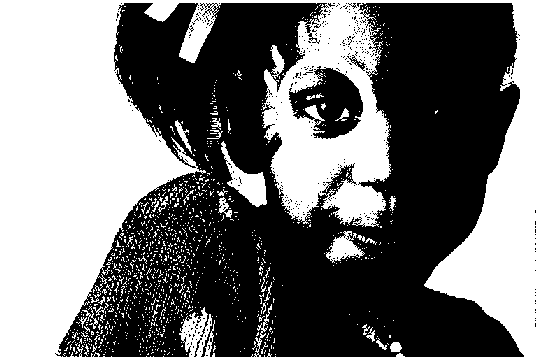
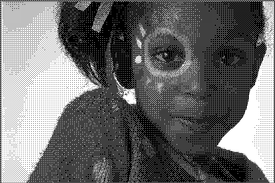
Figure 17.3 shows an example of conversion to a binary image via thresholding, using T=80.

It can be seen in Figure 17.3 that the binary image is not “shaded” properly–an artifact known as false contouring. False contouring occurs when quantizing at low bit rates (one bit in this case) because the quantization error is dependent upon the input signal. If one reduces this dependence, the visual quality of the binary image is usually enhanced.

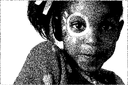
One method of reducing the signal dependence on the quantization error is to add uniformly distributed white noise to the input image prior to quantization. To each pixel of the gray scale image f(i,j), a white random number n in the range [–A,A] is added, and then the resulting image is quantized by a one-bit quantizer, as in Equation 17.3. The result of this method is illustrated in Figure 17.4, where the additive noise is uniform over [–40,40]. Notice that even though the resulting binary image is somewhat noisy, the false contouring has been significantly reduced.

Figure 17.4. 

Random noise binarization.

Halftone images are binary images that appear to have a gray scale rendition. Although the random thresholding technique described in "Binary Images" can be used to produce a halftone image, it is not often used in real applications since it yields very noisy results. In this section, we will describe a better halftoning technique known as ordered dithering.

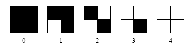
The human visual system tends to average a region around a pixel instead of treating each pixel individually, thus it is possible to create the illusion of many gray levels in a binary image, even though there are actually only two gray levels. With 2×2 binary pixel grids, we can represent 5 different “effective” intensity levels, as shown in Figure 17.5. Similarly for 3×3 grids, we can represent 10 distinct gray levels. In dithering, we replace blocks of the original image with these types of binary grid patterns.

Figure 17.5. 

Five different patterns of 2×2 binary pixel grids.

Remember from "Binary Images" that false contouring artifacts can be reduced if we can reduce the signal dependence or the quantization error. We showed that adding uniform noise to the monochrome image can be used to achieve this decorrelation. An alternative method would be to use a variable threshold value for the quantization process.

Ordered dithering consists of comparing blocks of the original image to a 2-D grid, known as a dither pattern. Each element of the block is then quantized using the corresponding value in the dither pattern as a threshold. The values in the dither matrix are fixed, but are typically different from each other. Because the threshold value varies between adjacent pixels, some decorrelation from the quantization error is achieved, which has the effect of reducing false contouring.

The following is an example of a 2×2 dither matrix,

(17.4)

This is a part of a general class of optimum dither patterns known as Bayer matrices. The values of the threshold matrix T(i,j) are determined by the order that pixels turn "ON". The order can be put in the form of an index matrix. For a Bayer matrix of size 2, the index matrix I(i,j) is given by

(17.5)

and the relation between T(i,j) and I(i,j) is given by

(17.6)

where n² is the total number of elements in the matrix.

Figure 17.6 shows the halftone image produced by Bayer dithering of size 4. It is clear from the figure that the halftone image provides good detail rendition. However the inherent square grid patterns are visible in the halftone image.

Figure 

Page 1Page 2Page 3Page 4Page 5Page 6Page 7Page 8Page 9Page 10Page 11Page 12Page 13Page 14Page 15Page 16Page 17Page 18Page 19Page 20Page 21Page 22Page 23Page 24

PREV   NEXT