Questions or comments concerning this laboratory should be directed to Prof. Charles A. Bouman, School of Electrical and Computer Engineering, Purdue University, West Lafayette IN 47907; (765) 494-0340; bouman@ecn.purdue.edu
This is the first part of a two week experiment in image processing. During this week, we will cover the fundamentals of digital monochrome images, intensity histograms, pointwise transformations, gamma correction, and image enhancement based on filtering.
In the second week , we will cover some fundamental concepts of color images. This will include a brief description on how humans perceive color, followed by descriptions of two standard color spaces. The second week will also discuss an application known as image halftoning.
An image is the optical representation of objects illuminated by a light source. Since we want to process images using a computer, we represent them as functions of discrete spatial variables. For monochrome (black-and-white) images, a scalar function f(i,j) can be used to represent the light intensity at each spatial coordinate (i,j). Figure 16.1 illustrates the convention we will use for spatial coordinates to represent images.
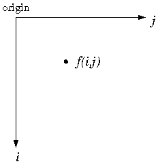
If we assume the coordinates to be a set of positive integers, for example i=1,⋯,M and j=1,⋯,N, then an image can be conveniently represented by a matrix.

We call this an M×N image, and the elements of the matrix are known as pixels.
The pixels in digital images usually take on integer values in the finite range,
where 0 represents the minimum intensity level (black), and Lmax
is the maximum intensity level (white) that the digital image can take on.
The interval  is known as a gray scale.
In this lab, we will concentrate on 8-bit images, meaning that each pixel is represented by a single byte. Since a byte can take on 256 distinct values, Lmax is 255 for an 8-bit image.
Download the file yacht.tif for the following section. Click here for help on the Matlab image command.
In order to process images within Matlab, we need to first understand their numerical representation. Download the image file yacht.tif . This is an 8-bit monochrome image. Read it into a matrix using
A = imread('yacht.tif');
Type whos
to display your variables.
Notice under the "Class" column that the A matrix
elements are of type uint8 (unsigned integer, 8 bits).
This means that Matlab is using a single byte to represent each pixel.
Matlab cannot perform numerical computation on numbers of type
uint8, so we usually need to convert the matrix to a floating point
representation.
Create a double precision representation of the image using
B = double(A);
.
Again, type whos
and notice the difference in the number
of bytes between A and B.
In future sections, we will be performing computations on our images,
so we need to remember to convert them to type
double before processing them.
Display yacht.tif using the following sequence of commands:
image(B);
colormap(gray(256));
axis('image');
The image command works for both type uint8 and
double images.
The colormap command specifies the range of displayed gray levels,
assigning black to 0 and white to 255.
It is important to note that if any pixel values are outside the range
0 to 255 (after processing), they will be clipped to 0 or 255 respectively
in the displayed image.
It is also important to note that a floating point pixel value will be
rounded down ("floored") to an integer before it is displayed.
Therefore the maximum number of gray levels that will be displayed on
the monitor is 255, even if the image values take on a continuous range.
Now we will practice some simple operations on the yacht.tif image. Make a horizontally flipped version of the image by reversing the order of each column. Similarly, create a vertically flipped image. Print your results.
Now, create a "negative" of the image by subtracting each pixel from 255 (here's an example of where conversion to double is necessary.) Print the result.
Finally, multiply each pixel of the original image by 1.5, and print the result.
Hand in two flipped images.
Hand in the negative image.
Hand in the image multiplied by factor of 1.5. What effect did this have?
Download the files house.tif and narrow.tif for the following sections.
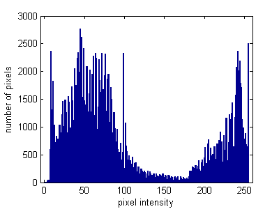
The histogram of a digital image shows how its pixel intensities are distributed. The pixel intensities vary along the horizontal axis, and the number of pixels at each intensity is plotted vertically, usually as a bar graph. A typical histogram of an 8-bit image is shown in Figure 16.2.
Write a simple Matlab function Hist(A)
which will plot the histogram of image matrix A.
You may use Matlab's hist function, however that function requires
a vector as input.
An example of using hist to plot a histogram of a matrix would be
x=reshape(A,1,M*N);
hist(x,0:255);
where A is an image, and M and N are the number of rows and columns in A.
The reshape command is creating a row vector out of the image matrix,
and the hist command plots a histogram with bins centered at [0:255].
Download the image file
house.tif
,
and read it into Matlab.
Test your Hist function on the image. Label the axes of
the histogram and give it a title.
Hand in your labeled histogram. Comment on the distribution of the pixel intensities.
A pointwise transformation is a function that maps pixels from
one intensity to another.
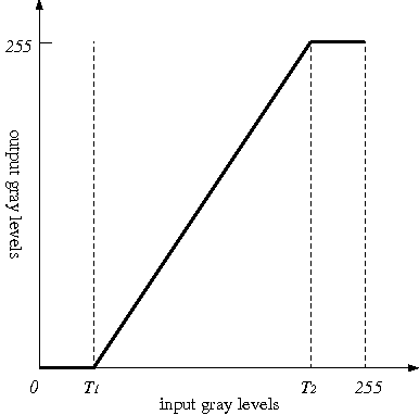
An example is shown in Figure 16.3.
The horizontal axis shows all possible intensities
of the original image, and the vertical axis shows the intensities
of the transformed image. This particular transformation maps the
"darker" pixels in the range  to a level of zero (black),
and similarly maps the "lighter" pixels in
to a level of zero (black),
and similarly maps the "lighter" pixels in  to white.
Then the pixels in the range
to white.
Then the pixels in the range  are "stretched out" to
use the full scale of [0,255]. This can have the effect of
increasing the contrast in an image.
are "stretched out" to
use the full scale of [0,255]. This can have the effect of
increasing the contrast in an image.
Pointwise transformations will obviously affect the pixel distribution, hence they will change the shape of the histogram. If a pixel transformation can be described by a one-to-one function, y=f(x), then it can be shown that the input and output histograms are approximately related by the following:

Since x and y need to be integers in Equation 16.3, the evaluation of x=f–1(y) needs to be rounded to the nearest integer.
The pixel transformation shown in Figure 16.3 is not a
one-to-one function. However, Equation 16.3 still may be
used to give insight into the effect of the transformation. Since the
regions  and
and  map to the single points 0 and 255,
we might expect "spikes" at the points 0 and 255 in the
output histogram.
The region [1,254] of the output histogram will be directly
related to the input histogram through Equation 16.3.
map to the single points 0 and 255,
we might expect "spikes" at the points 0 and 255 in the
output histogram.
The region [1,254] of the output histogram will be directly
related to the input histogram through Equation 16.3.
First, notice from x=f–1(y) that the region [1,254] of the output
is being mapped from the region  of the input.
Then notice that f'(x) will be a constant scaling factor throughout the
entire region of interest. Therefore, the output histogram should
approximately be a stretched and rescaled version of the input
histogram, with possible spikes at the endpoints.
of the input.
Then notice that f'(x) will be a constant scaling factor throughout the
entire region of interest. Therefore, the output histogram should
approximately be a stretched and rescaled version of the input
histogram, with possible spikes at the endpoints.
Write a Matlab function that will perform the pixel transformation shown in Figure 16.3. It should have the syntax
output = pointTrans(input, T1, T2) .
Determine an equation for the graph in Figure 16.3, and use this in your function. Notice you have three input regions to consider. You may want to create a separate function to apply this equation.
If your function performs the transformation one pixel at a time, be sure to allocate the space for the output image at the beginning to speed things up.
Download the image file narrow.tif and read it into Matlab. Display the image, and compute its histogram. The reason the image appears "washed out" is that it has a narrow histogram. Print out this picture and its histogram.
Now use your pointTrans function to spread out the histogram using
T1=70 and T2=180. Display the new image and its histogram.
(You can open another figure window using the figure command.)
Do you notice a difference in the "quality" of the picture?
Hand in your code for pointTrans.
Hand in the original image and its histogram.
Hand in the transformed image and its histogram.
What qualitative effect did the transformation have on the original image? Do you observe any negative effects of the transformation?
Compare the histograms of the original and transformed images. Why are there zeros in the output histogram?
Download the file dark.tif for the following section.
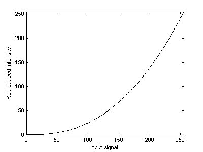
The light intensity generated by a physical device is usually a nonlinear function of the original signal. For example, a pixel that has a gray level of 200 will not be twice as bright as a pixel with a level of 100. Almost all computer monitors have a power law response to their applied voltage. For a typical cathode ray tube (CRT), the brightness of the illuminated phosphors is approximately equal to the applied voltage raised to a power of 2.5. The numerical value of this exponent is known as the gamma (γ) of the CRT. Therefore the power law is expressed as
where I is the pixel intensity and V is the voltage applied to the device.
If we relate Equation 16.4 to the pixel values for an 8-bit image, we get the following relationship,

where x is the original pixel value, and y is the pixel intensity as it appears on the display. This relationship is illustrated in Figure 16.4.
In order to achieve the correct reproduction of intensity, this nonlinearity must be compensated by a process known as γcorrection. Images that are not properly corrected usually appear too light or too dark. If the value of γ is available, then the correction process consists of applying the inverse of Equation 16.5. This is a straightforward pixel transformation, as we discussed in the section "Pointwise Transformations".
Write a Matlab function that will γ correct an image by applying the inverse of Equation 16.5. The syntax should be
B = gammCorr(A,gamma)
where A is the uncorrected image, gamma is the γ of the device, and B is the corrected image. (See the hints in "Pointwise Transformations".)
The file dark.tif is an image that has not been γ corrected for your monitor. Download this image, and read it into Matlab. Display it and observe the quality of the image.
Assume that the γ for your monitor is 2.2.
Use your gammCorr function to
correct the image for your monitor, and display the
resultant image. Did it improve the quality of the picture?
Hand in your code for gammCorr.
Hand in the γ corrected image.
How did the correction affect the image? Does this appear to be the correct value for γ ?
Sometimes, we need to process images to improve their appearance. In this section, we will discuss two fundamental image enhancement techniques: image smoothing and sharpening.
Smoothing operations are used primarily for diminishing spurious effects that may be present in a digital image, possibly as a result of a poor sampling system or a noisy transmission channel. Lowpass filtering is a popular technique of image smoothing.
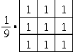
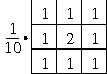
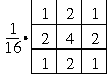
Some filters can be represented as a 2-D convolution of an image f(i,j) with the filter's impulse response h(i,j).

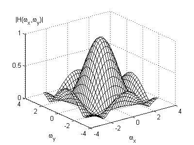
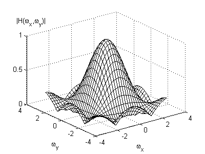
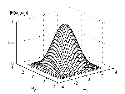
Some typical lowpass filter impulse responses are shown in Figure 16.5, where the center element corresponds to h(0,0). Notice that the terms of each filter sum to one. This prevents amplification of the DC component of the original image. The frequency response of each of these filters is shown in Figure 16.6.