Questions or comments concerning this laboratory should be directed to Prof. Charles A. Bouman, School of Electrical and Computer Engineering, Purdue University, West Lafayette IN 47907; (765) 494-0340; bouman@ecn.purdue.edu
A discrete-time system is anything that takes a discrete-time signal as input and generates a discrete-time signal as output.[1] The concept of a system is very general. It may be used to model the response of an audio equalizer or the performance of the US economy.
In electrical engineering, continuous-time signals are usually processed by electrical circuits described by differential equations. For example, any circuit of resistors, capacitors and inductors can be analyzed using mesh analysis to yield a system of differential equations. The voltages and currents in the circuit may then be computed by solving the equations.
The processing of discrete-time signals is performed by discrete-time systems. Similar to the continuous-time case, we may represent a discrete-time system either by a set of difference equations or by a block diagram of its implementation. For example, consider the following difference equation.
This equation represents a discrete-time system. It operates on the input signal x(n) to produce the output signal y(n). This system may also be defined by a system diagram as in Figure 3.1.
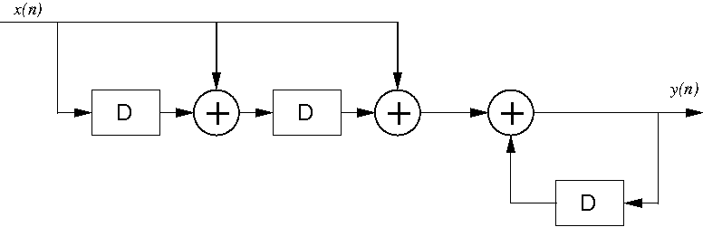
Mathematically, we use the notation y=S[x] to denote a discrete-time system S with input signal x(n) and output signal y(n). Notice that the input and output to the system are the complete signals for all time n. This is important since the output at a particular time can be a function of past, present and future values of x(n).
It is usually quite straightforward to write a computer program to implement a discrete-time system from its difference equation. In fact, programmable computers are one of the easiest and most cost effective ways of implementing discrete-time systems.
While equation Equation 3.1 is an example of a linear time-invariant system, other discrete-time systems may be nonlinear and/or time varying. In order to understand discrete-time systems, it is important to first understand their classification into categories of linear/nonlinear, time-invariant/time-varying, causal/noncausal, memoryless/with-memory, and stable/unstable. Then it is possible to study the properties of restricted classes of systems, such as discrete-time systems which are linear, time-invariant and stable.
Submit these background exercises with the lab report.
Discrete-time digital systems are often used in place of analog processing systems. Common examples are the replacement of photographs with digital images, and conventional NTSC TV with direct broadcast digital TV. These digital systems can provide higher quality and/or lower cost through the use of standardized, high-volume digital processors.
The following two continuous-time systems are commonly used in electrical engineering:

For each of these two systems, do the following:
| i.: Formulate a discrete-time system that approximates the continuous-time function. |
| ii.: Write down the difference equation that describes your discrete-time system. Your difference equation should be in closed form, i.e. no summations. |
| iii.: Draw a block diagram of your discrete-time system as in Figure 3.1. |
One reason that digital signal processing (DSP) techniques are so powerful is that they can be used for very different kinds of signals. While most continuous-time systems only process voltage and current signals, a computer can process discrete-time signals which are essentially just sequences of numbers. Therefore DSP may be used in a very wide range of applications. Let's look at an example.
A stockbroker wants to see whether the average value of a certain stock is increasing or decreasing. To do this, the daily fluctuations of the stock values must be eliminated. A popular business magazine recommends three possible methods for computing this average.


Do the following:
For each of the these three methods: 1) write a difference equation, 2) draw a system diagram, and 3) calculate the impulse response.
Explain why methods Equation 3.3 and Equation 3.5 are known as moving averages.
Write two Matlab functions that will apply the differentiator and integrator systems, designed in the "Example Discrete-time Systems" section, to arbitrary input signals. Then apply the differentiator and integrator to the following two signals for –10≤n≤20.
δ ( n ) – δ ( n – 5 )
u(n)–u(n–(N+1)) with N=10
Hint:
To compute the function u(n) for –10≤n≤20,
first set n = -10:20, and then use the
Boolean expression u = (n>=0).
For each of the four cases, use the subplot and stem commands to plot each input and output signal on a single figure.
Submit printouts of your Matlab code and hardcopies containing the input and output signals. Discuss the stability of these systems.
In this section, we will study the effect of two discrete-time filters. The first filter, y=S1[x], obeys the difference equation

and the second filter, y=S2[x], obeys the difference equation

Write Matlab functions to implement each of these filters.
In Matlab, when implementing a difference equation using a loop
structure, it is very good practice to pre-define your output vector before
entering into the loop.
Otherwise, Matlab has to resize the output vector at each iteration.
For example, say you are using a FOR loop to filter the signal
x(n),
yielding an output
y(n).
You can pre-define the output vector by issuing the command
y=zeros(1,N) before entering the loop,
where N is the final length of y.
For long signals, this speeds up the computation dramatically.
Now use these functions to calculate the impulse response of each of the
following 5 systems: S1, S2,
 (i.e., the series connection with S1 following S2),
 (i.e., the series connection with S2 following S1),
and S1+S2.
(i.e., the series connection with S2 following S1),
and S1+S2.
For each of the five systems, draw and submit a system diagram (use only delays, multiplications and additions as in Figure 3.1). Also submit plots of each impulse response. Discuss your observations.
For this section download the music.au file. For help on how to play audio signals click here.
Use the command auread to load the file
music.au into Matlab.
Then use the Matlab function sound to listen to the signal.
Next filter the audio signal with each of the two systems S1 and S2 from the previous section. Listen to the two filtered signals.
How do the filters change the sound of the audio signals? Explain your observations.
Consider the system y=S2[x]
from the "Difference Equations" section.
Find a difference equation for a new
system y=S3[x] such that
 where δ
denotes the discrete-time impulse function δ(n).
Since both systems S2 and S3 are LTI, the time-invariance
and superposition properties can be used to obtain
where δ
denotes the discrete-time impulse function δ(n).
Since both systems S2 and S3 are LTI, the time-invariance
and superposition properties can be used to obtain
 for any discrete-time signal x.
We say that the systems S3
and S2 are inverse filters because
they cancel out the effects of each other.
for any discrete-time signal x.
We say that the systems S3
and S2 are inverse filters because
they cancel out the effects of each other.
Hint: The system y=S3[x] can be described by the difference equation

where a and b are constants.
Write a Matlab function y = S3(x)
which implements
the system S3.
Then obtain the impulse response of both S3
and S3[S2[δ]].
Draw a system diagram for the system S3, and submit plots of the impulse responses for S3 and S3(S2).
For this section download the zip file bbox.zip.
Often it is necessary to determine if a system is linear and/or time-invariant. If the inner workings of a system are not known, this task is impossible because the linearity and time-invariance properties must hold true for all possible inputs signals. However, it is possible to show that a system is non-linear or time-varying because only a single instance must be found where the properties are violated.
The zip file bbox.zip
contains three "black-box" systems in the files bbox1.p,
bbox2.p, and bbox3.p.
These files work as Matlab functions, with the syntax
y=bboxN(x), where x and y are the input and the output signals, and
N = 1, 2 or 3.
Exactly one of these systems is non-linear, and exactly one of
them is time-varying.
Your task is to find the non-linear system and the time-varying
system.
You should try a variety of input signals until you find a counter-example.
When testing for time-invariance, you need to look at the responses to a signal and to its delayed version. Since all your signals in MATLAB have finite duration, you should be very careful about shifting signals. In particular, if you want to shift a signal x by M samples to the left, x should start with at least M zeros. If you want to shift x by M samples to the right, x should end with at least M zeros.
When testing for linearity, you may find that simple inputs such as
the unit impulse do not accomplish the task. In this case, you should
try something more complicated like a sinusoid or a random signal
generated with the random command.
State which system is non-linear, and which system is time-varying. Submit plots of input/output signal pairs that support your conclusions. Indicate on the plots why they support your conclusions.
For this section download stockrates.mat. For help on loading Matlab files click here.
Load stockrates.mat into Matlab. This file contains a vector, called rate, of daily stock market exchange rates for a publicly traded stock.
Apply filters
Equation 3.4 and Equation 3.5
from the "Stock Market Example" section of the background exercises to smooth the stock values.
When you apply the filter of Equation 3.4 you will need
to initialize the value of avgvalue(yesterday).
Use an initial value of 0.
Similarly, in Equation 3.5, set the initial values of
the "value" vector to 0 (for the days prior to the start of data collection).
Use the subplot command to plot the original stock values,
the result of filtering with Equation 3.4,
and the result of filtering with Equation 3.5.
Submit your plots of the original and filtered exchange-rates. Discuss the advantages and disadvantages of the two filters. Can you suggest a better method for initializing the filter outputs?