Questions or comments concerning this laboratory should be directed to Prof. Charles A. Bouman, School of Electrical and Computer Engineering, Purdue University, West Lafayette IN 47907; (765) 494-0340; bouman@ecn.purdue.edu
In this experiment,we will use Fourier series and Fourier transforms to analyze continuous-time and discrete-time signals and systems. The Fourier representations of signals involve the decomposition of the signal in terms of complex exponential functions. These decompositions are very important in the analysis of linear time-invariant (LTI) systems, due to the property that the response of an LTI system to a complex exponential input is a complex exponential of the same frequency! Only the amplitude and phase of the input signal are changed. Therefore, studying the frequency response of an LTI system gives complete insight into its behavior.
In this experiment and others to follow, we will use the Simulink extension to Matlab. Simulink is an icon-driven dynamic simulation package that allows the user to represent a system or a process by a block diagram. Once the representation is completed, Simulink may be used to digitally simulate the behavior of the continuous or discrete-time system. Simulink inputs can be Matlab variables from the workspace, or waveforms or sequences generated by Simulink itself. These Simulink-generated inputs can represent continuous-time or discrete-time sources. The behavior of the simulated system can be monitored using Simulink's version of common lab instruments, such as scopes, spectrum analyzers and network analyzers.
Submit these background exercises with the lab report.
Each signal given below represents one period of a periodic signal with period T0.
Period T0=2. For t∈[0,2]:

Period T0=1. For  :
:

For each of these two signals, do the following:
| i: Compute the Fourier series expansion in
the form
(4.1)
where f0=1/T0 .
 Hint
You may want to use one of the following references:
Sec. 4.1 of ``Digital Signal Processing'', by Proakis and Manolakis, 1996;
Sec. 4.2 of ``Signals and Systems'', by Oppenheim and Willsky, 1983;
Sec. 3.3 of ``Signals and Systems'', Oppenheim and Willsky, 1997.
Note that in the expression above, the function in the summation is
|
ii: Sketch the signal on the interval  . .
|
For the discrete-time system described by the following difference equation,
| i: Compute the impulse response. |
| ii: Draw a system diagram. |
| iii: Take the Z-transform of the difference equation using the linearity and the time shifting properties of the Z-transform. |
| iv: Find the transfer function, defined as
(4.3)  |
v: Use Matlab to compute and plot the magnitude and phase responses,
 and and  ,
for –π<ω<π .
You may use Matlab commands ,
for –π<ω<π .
You may use Matlab commands phase and abs.
|
In this section, we will learn the basics of Simulink and build a simple system.
For help on "Simulink" click here. For the following sections download the file Lab3Utilities.zip.
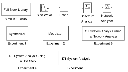
To get the library of Simulink functions for this laboratory, download the file Lab3Utilities.zip. Once Matlab is started, type “Lab3” to bring up the library of Simulink components shown in Figure 4.1. This library contains a full library of Simulink blocks, a spectrum analyzer and network analyzer designed for this laboratory, a sine wave generator, a scope, and pre-design systems for each of the experiments that you will be running.
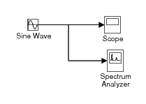
In order to familiarize yourself with Simulink, you will first build the system shown in Figure 4.2. This system consists of a sine wave generator that feeds a scope and a spectrum analyzer.
Open a window for a new system by using the New option
from the File pull-down menu, and select Model.
Drag the Sine Wave, Scope,
and Spectrum Analyzer blocks
from the Lab3 window into the new window you created.
Now you need to connect these three blocks.
With the left mouse button, click on the output of the Sine Wave
and drag it to the input of the Scope.
Now use the right button to click on the line you just created, and drag
to the input of the Spectrum Analyzer block.
Your system should now look like Figure 4.2.
Double click on the Scope block to make the plotting
window for the scope appear.
Set the simulation parameters by selecting Configuration Parameters
from
the Simulation pull-down menu. Under the Solver tab, set the
Stop time to 50, and the Max step size to 0.02. Then select
OK. This will
allow the Spectrum Analyzer to make a more accurate calculation.
Start the simulation by using the Start option from
the Simulation pull-down menu.
A standard Matlab figure window will pop up showing
the output of the Spectrum Analyzer.
Change the frequency of the sine wave to 5*pi rad/sec
by double clicking on the Sine Wave icon and changing the
number in the Frequency field.
Restart the simulation. Observe the change in the waveform and
its spectral density. If you want to change the time scaling in the plot
generated by the spectrum analyzer, from the Matlab prompt use the
subplot(2,1,1)
and axis()
commands.
When you are done, close the system window you created
by using the Close option
from the File pull-down menu.
For help on the following topics select the corresponding link: simulink or printing figures in Simulink.
In this section, we will study the use and properties of the continuous-time Fourier transform with Simulink. The Simulink package is especially useful for continuous-time systems because it allows the simulation of their behavior on a digital computer.
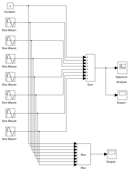
Double click the icon labeled Synthesizer
to bring up a model as shown in Figure 4.3.
This system may be used to synthesize periodic signals by
adding together the harmonic components of a Fourier series
expansion.
Each Sin Wave block can be set to a specific frequency,
amplitude and phase.
The initial settings of the Sin Wave blocks are set
to generate the Fourier series expansion

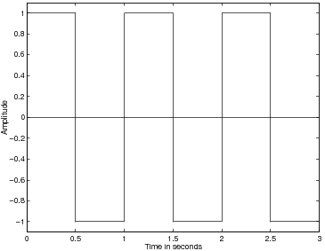
These are the first 8 terms in the Fourier series of the periodic square wave shown in Figure 4.4.
Run the model by selecting Start
under the Simulation menu.
A graph will pop up that shows the synthesized square wave signal
and its spectrum.
This is the output of the Spectrum Analyzer.
After the simulation runs for a while,
the Spectrum Analyzer element will update
the plot of the spectral energy and the incoming waveform.
Notice that the energy is concentrated in peaks corresponding
to the individual sine waves.
Print the output of the Spectrum Analyzer.
You may have a closer look at the synthesized signal
by double clicking on the Scope1 icon.
You can also see a plot of all the individual sine waves
by double clicking on the Scope2 icon.
Synthesize the two periodic waveforms defined in the
"Synthesis of Periodic Signals" section of the background exercises.
Do this by setting the frequency, amplitude, and phase
of each sinewave generator to the proper values.
For each case, print the output of the Spectrum Analyzer.
Hand in plots of the Spectrum Analyzer output
for each of the three synthesized waveforms.
For each case, comment on how the synthesized waveform
differs from the desired signal, and on the structure
of the spectral density.
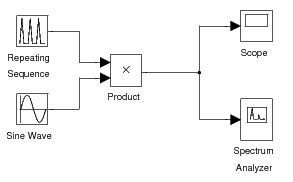
Double click the icon labeled Modulator
to bring up a system as shown in Figure 4.5.
This system modulates a triangular pulse signal with a sine wave.
You can control the duration and duty cycle of the triangular
envelope and the frequency of the modulating sine wave.
The system also contains a spectrum analyzer which plots
the modulated signal and its spectrum.
Generate the following signals by adjusting the Time values and
Output values of the Repeating Sequence block and the
Frequency of the Sine Wave. The Time values vector
contains entries spanning one period of the repeating signal.
The Output values vector
contains the values of the repeating signal at the times specified
in the Time values vector. Note that the Repeating Sequence block
does NOT create a discrete time signal. It creates a continuous time signal
by connecting the output values with line segments.
Print the output of the Spectrum Analyzer for each signal.
Triangular pulse duration of 1 sec; period of 2 sec; modulating frequency of 10 Hz (initial settings of the experiment).
Triangular pulse duration of 1 sec; period of 2 sec; modulating frequency of 15 Hz.
Triangular pulse duration of 1 sec; period of 3 sec; modulating frequency of 10 Hz.
Triangular pulse duration of 1 sec; period of 6 sec; modulating frequency of 10 Hz.
Notice that the spectrum of the modulated signal consists of of a comb of impulses in the frequency domain, arranged around a center frequency.
Hand in plots of the output of the Spectrum Analyzer
for each signal.
Answer following questions:
1) What effect does changing the modulating frequency
have on the spectral density?
2) Why does the spectrum have a comb structure and what
is the spectral distance between impulses? Why?
3) What would happen to the spectral density if the period of the
triangle pulse were to increase toward infinity? (in the limit)
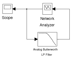
Double click the icon labeled
CT System Analysis using a Network Analyzer
to bring up a system as shown in Figure 4.6.
This system includes a Network Analyzer model
for measuring the frequency response of a system.
The Network Analyzer works by generating a weighted
chirp signal (shown on the Scope)
as an input to the system-under-test.
The analyzer measures the frequency response of the input
and output of the system and computes the transfer function.
By computing the inverse Fourier transform, it then
computes the impulse response of the system.
Use this setup to compute the frequency and impulse
response of the given fourth order Butterworth filter with a cut-off
frequency of 1Hz. Print the figure showing the magnitude response,
the phase response and the impulse response of the system. To use the tall
mode to obtain a larger printout, type orient('tall'); directly before you print.
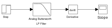
An alternative method for computing the impulse response is
to input a step into the system and then to compute the derivative
of the output.
The model for doing this is given in the
CT System Analysis using a Unit Step block.
Double click on this icon and compute the impulse response of the
filter using this setup (Figure 4.7).
Make sure that the characteristics of the filter
are the same as in the previous setup.
After running the simulation, print the graph
of the impulse response.
Hand in the printout of the output of the Network Analyzer
(magnitude and phase of the frequency response, and the
impulse response) and the plot of the impulse response
obtained using a unit step.
What are the advantages and disadvantages of each method?
In this section of the laboratory, we will study the use of the discrete-time Fourier transform.
The DTFT (Discrete-Time Fourier Transform) is the Fourier representation used
for finite energy discrete-time signals.
For a discrete-time signal, x(n), we denote the DTFT as the
function  given by the expression

Since  is a periodic function of ω
with a period of 2π, we need only to compute
is a periodic function of ω
with a period of 2π, we need only to compute  for
–π<ω<π .
for
–π<ω<π .
Write a Matlab function X=DTFT(x,n0,dw)
that computes the DTFT
of the discrete-time signal x
Here n0 is the time index
corresponding to the 1st element of the x
vector, and dw is the spacing between the samples
of the Matlab vector X.
For example, if x
is a vector of length N, then
its DTFT is computed by

where w is a vector of values formed by w=(-pi:dw:pi)
.
In Matlab, j or i is defined
as  . However, you may also compute this value using
the Matlab expression
. However, you may also compute this value using
the Matlab expression i=sqrt(-1).
For the following signals use your DTFT function to
i: Compute  |
ii: Plot the magnitude and the phase of  in a single
plot using the in a single
plot using the subplot command.
|
Use the abs()
and angle()
commands.
