The Merrian-Webster dictionary defines a signal as:
A detectable physical quantity or impulse (as a voltage, current, or magnetic field strength) by which messages or information can be transmitted.
These are the types of signals which will be of interest in this book. Indeed, signals are not only the means by which we perceive the world around us, they also enable individuals to communicate with one another on a massive scale. So while our primary emphasis in this book will be on the theoretical foundations of signal processing, we will also try to give examples of the tremendous impact that signals and systems have on society. We will focus on two broad classes of signals, discrete-time and continuous-time. We will consider discrete-time signals later on in this book. For now, we will focus our attention on continuous-time signals. Fortunately, continuous-time signals have a very convenient mathematical representation. We represent a continuous-time signal as a function x(t) of the real variable t. Here, t represents continuous time and we can assign to t any unit of time we deem appropriate (seconds, hours, years, etc.). We do not have to make any particular assumptions about x(t) such as boundedness (a signal is bounded if it has a finite value). Some of the signals we will work with are in fact, not bounded (i.e. they take on an infinite value). However most of the continuous-time signals we will deal with in the real world are bounded.
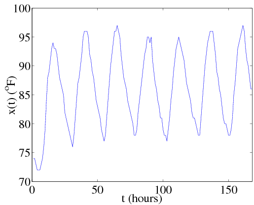
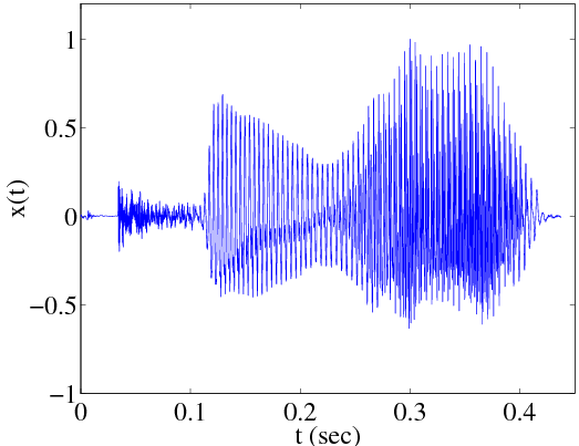
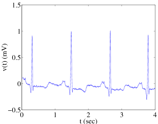
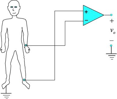
We actually encounter signals every day. Suppose we sketch a graph of the temperature outside the Jerry Junkins Electrical Engineering Building on the SMU campus as a function of time. The graph might look something like in Figure 1.1. This is an example of a signal which represents the physical quantity temperature as it changes with time during the course of a week. Figure 1.2 shows another common signal, the speech signal. Human speech signals are often measured by converting sound (pressure) waves into an electrical potential using a microphone. The speech signal therefore corresponds to the air pressure measured at the point in space where the microphone was located when the speech was recorded. The large deviations which the speech signal undergoes corresponds to vowel sounds such as “ahhh" or “eeeeh" (voiced sounds) while the smaller portions correspond to sounds such as “th" or “sh" (unvoiced sounds). In Figure 1.3, we see yet another signal called an electrocardiogram (EKG). The EKG is a voltage which is generated by the heart and measured by subtracting the voltage recorded from two points on the human body as seen in Figure 1.4. Since the heart generates very low-level voltages, the difference signal must be amplified by a high-gain amplifier.
Signals can be characterized in several different ways. Audio signals (music, speech, and really, any kind of sound we can hear) are particularly useful because we can use our existing notion of “loudness" and “pitch" which we normally associate with an audio signal to develop ways of characterizing any kind of signal. In terms of audio signals, we use “power" to characterize the loudness of a sound. Audio signals which have greater power sound “louder" than signals which have lower power (assuming the pitch of the sounds are within the range of human hearing). Of course, power is related to the amplitude, or size of the signal. We can develop a more precise definition of power. The signal power is defined as:

The energy of this signal is similarly defined
We can see that power has units of energy per unit time. Strictly speaking, the units for energy depend on the units assigned to the signal. If x(t) is a voltage, than the units for ex would be volts2-seconds. Notice also that some signals may not have finite energy. As we will see shortly, periodic signals do not have finite energy. Signals having a finite energy are sometimes called energy signals. Some signals that have infinite energy however can have finite power. Such signals are sometimes called power signals.
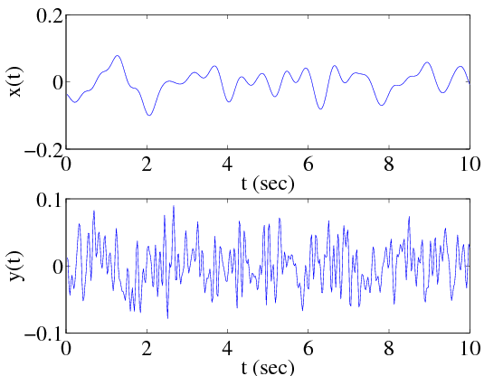
We use the concept of “frequency" to characterize the pitch of audio signals. The frequency of a signal is closely related to the variation of the signal with time. Signals which change rapidly with time have higher frequencies than signals which are changing slowly with time as seen Figure 1.5. As we shall see, signals can also be represented in terms of their frequencies, X(jΩ), where Ω is a frequency variable. Devices which enable us to view the frequency content of a signal in real-time are called spectrum analyzers.
Something to keep in mind is that the signals shown in Figures Figure 1.1, Figure 1.2, and Figure 1.3 each have different units (degrees Fahrenheit, pressure, and voltage, respectively). So while we can compare relative frequencies between these signals, it doesn't make much sense to compare their power since each signal has different units. We will take a more formal look at the frequency of signals starting in Chapter 2.
We will be considering the following basic operations on signals:
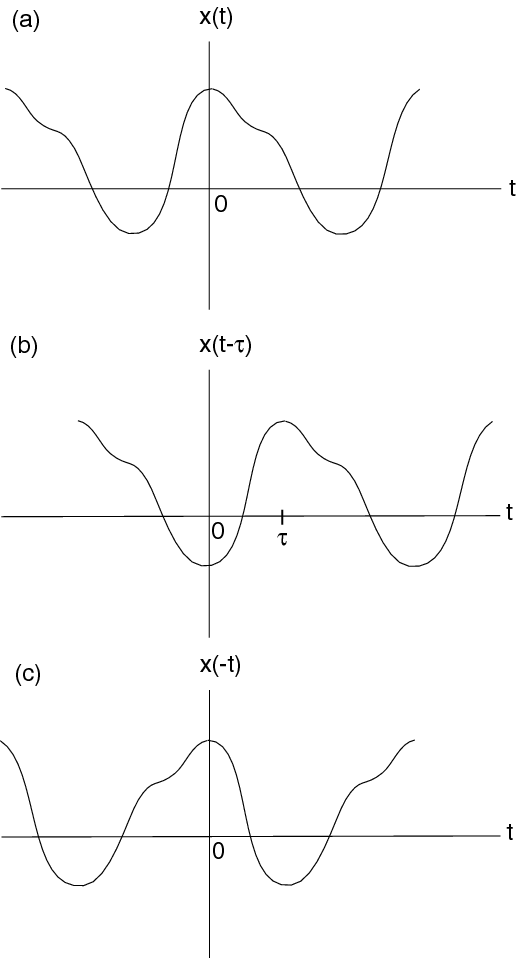
Time shifting:
The effect that a time shift has on the appearance of a signal is seen in Figure 1.6. If τ is a positive number, the time shifted signal, x(t–τ) gets shifted to the right, otherwise it gets shifted left.
Time reversal:
Time reversal flips the signal about t=0 as seen in Figure 1.6.
Addition: any two signals can be added to form a third signal,
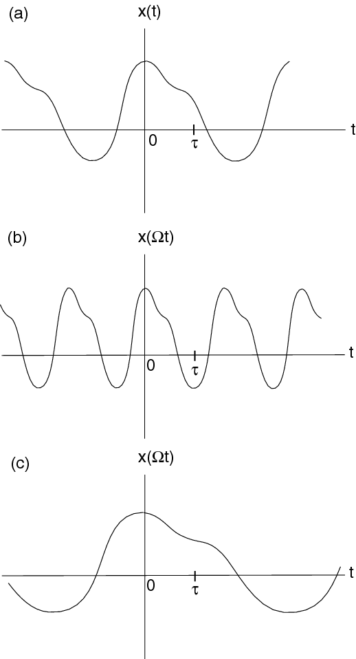
Time scaling:
Time scaling “compresses" the signal if Ω>1 or “stretches" it if Ω<1 (see Figure 1.7).
Multiplication by a constant, α:
Multiplication of two signals, their product is also a signal.
Multiplication of signals has many useful applications in wireless communications.
Differentiation:

Integration:
There is another very important signal operation called convolution which we will look at in detail in Chapter 3. As we shall see, convolution is a combination of several of the above operations.
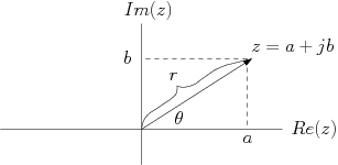
Before we begin studying signals, we need to review some basic aspects of complex numbers and complex arithmetic. The rectangular coordinate representation of a complex number z is z has the form:
where a and b are real numbers and  . The real
part of z is the number a, while the imaginary part of z
is the number b. We also note that jb(jb)=–b2 (a real number)
since j(j)=–1. Any number having the form
. The real
part of z is the number a, while the imaginary part of z
is the number b. We also note that jb(jb)=–b2 (a real number)
since j(j)=–1. Any number having the form
where b is a real number is an imaginary number. A complex number can also be represented in polar coordinates
where

is the magnitude and

is the phase of the complex number z. The notation for the magnitude and phase of a complex number is given by |z| and ∠z, respectively. Using Euler's Identity:
it follows that a=rcos(θ) and b=rsin(θ). Figure 1.8 illustrates how polar coordinates and rectangular coordinates are related.
Rectangular coordinates and polar coordinates are each useful depending on the type of mathematical operation performed on the complex numbers. Often, complex numbers are easier to add in rectangular coordinates, but multiplication and division is easier in polar coordinates. If z=a+jb is a complex number then its complex conjugate is defined by
in polar coordinates we have
note that zz*=|z|2=r2 and z+z*=2a. Also, if z1,z2,...,zN are complex numbers it can be easily shown that
and
Table 1.1 indicates how two complex numbers combine in terms of addition, multiplication, and division when expressed in rectangular and in polar coordinates.
| operation | rectangular | polar |
|
|