You may have noticed that we avoided taking the Fourier transform of a number of signals. For example, we did not try to compute the Fourier Transform of the unit step function, x(t)=u(t), or the ramp function x(t)=tu(t). The reason for this is that these signals do not have a Fourier transform that converges to a finite value for all Ω. Recall that in order to deal with periodic signals such as we had to settle for Fourier transforms having impulse functions in them. The Laplace transform gives us a mechanism for dealing with signals that do not have finite-valued Fourier Transforms.

The double-sided Laplace Transform of x(t) is defined as follows:

where we define

We observe that the Laplace transform is a generalization of the Fourier transform since

Therefore, we can write

The inverse Laplace transform can be derived using this idea. Applying the inverse Fourier transform to F{e^–σtx (t)} gives

(4.5)

Using Equation 4.2 leads to

(4.6)

Substituting s for Ω and solving for x(t) in Equation 4.5 gives

(4.7)

Equation Equation 4.7 is called the inverse Laplace transform. The integration is along a straight line in the complex s-plane corresponding to a fixed value of σ. This is illustrated in Figure 4.1.

Figure 4.1. 

The inverse Laplace transform integrates along a line having a constant σ in the complex s–plane.

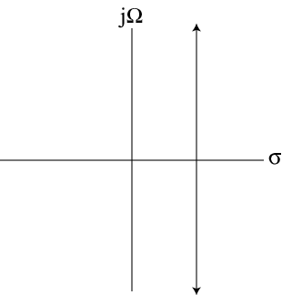
It is important that this line exist in a region of the s-plane that corresponds to the region of convergence for the Laplace transform. The region of convergence is defined as that region in the s-plane for which

Note that since s=σ+jΩ this is equivalent to

We define the single-sided Laplace transform as

where the lower limit of integration tacitly includes the point t=0. That is, 0^– represents a point just to the negative side of t=0. This allows for the integral to take into account signal features that occur at t=0 such as a step or impulse function. The single-sided Laplace transform is motivated by the fact that most signals are turned on at some point. If the region of convergence is not specified then different signals can yield identical double-sided Laplace transforms, as the following example illustrates.

Example 3.1 Consider the signal

The double-sided Laplace transform is given by

(4.12)

the magnitude of e^{–(σ+α)∞} is zero only if σ>–α which establishes the region of convergence. Therefore we have

(4.13)

Now consider the Laplace transform of the signal

We have

(4.15)

Here, the quantity e^(σ+α)∞ is zero only if σ<–α so we have

(4.16)

which is identical to X₁(s) except for the region of convergence.

To avoid scenarios where two different signals have the same double-sided Laplace transform, we restrict our signals to those which are assumed to be zero for t<0. Such signals are called causal signals.

The region of convergence for the single-sided Laplace transform is a region in the s-plane satisfying σ>σ_min as shown in Figure 4.2.

Figure 4.2. 

The region of convergence of the single-sided Laplace transform in the complex s–plane.

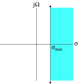
To see this, we observe that if

then it must be the case that

for σ>σ_min, since e^–σt decreases faster than e^–σ_mint. Finally, the inverse single-sided Laplace transform is the same as the inverse double-sided Laplace transform (see Equation 4.7), since a single sided Laplace transform can be interpreted as the double-sided Laplace transform of a signal satisfying x(t)=0,t<0. From here on, we will work exclusively with the single-sided Laplace transform. Unless we need to specifically differentiate between the single or double-sided transforms, we will refer to the single-sided Laplace transform as simply the “Laplace transform".

The properties associated with the Laplace transform are similar to those of the Fourier transform. First, let's set define some notation, we will use the notation L{} to denote the Laplace transform operation. Therefore we can write X(s)=L{x ( t )} and x(t)=L^–1{X ( s )} for the forward and inverse Laplace transforms, respectively. We can also use the transform pair notation used earlier:

With this notation defined, lets now look at some properties.

Time Delay

The reason we call this the time delay property rather than the time shift property is that the time shift must be positive, i.e. if τ>0, then x(t–τ) corresponds to a delay. If τ<0 then we would not be able to use the single-sided Laplace transform because we would have a lower integration limit of τ, which is less than zero. To derive the property, lets evaluate the Laplace transform of the time-delayed signal

(4.21) L {x ( t – τ )} = ∫₀^∞x ( t – τ ) e ^{– s t} d t

Letting γ=t–τ leads to t=γ+τ and dt=dγ. Substituting these quantities into Equation 4.21 gives

(4.22)

where we note that the first integral in the last line is zero since x(t)=0,t<0. Therefore the time delay property is given by

(4.23) L {x ( t – τ )} = e ^{– s τ} X ( s )

s-Shift

This property is the Laplace transform corresponds to the frequency shift property of the Fourier transform. In fact, the derivation of the s-shift property is virtually identical to that of the frequency shift property.

(4.24)

The s-shift property also alters the region of convergence of the Laplace transform. If the region of convergence for X(s) is σ>σ_min, then the region of convergence for L{e^–a