Two-dimensional flow of an incompressible, Newtonian fluid can be formulated with the stream function and vorticity as dependent variables.

(11.1)

We will begin developing a generic code by assuming steady, creeping (zero Reynolds number) flow with specified velocity on the boundaries in a rectangular domain. The PDE are now,

(11.2)

This is a pair of linear, elliptic PDEs. The boundary conditions with specified velocity are

(11.3)

The boundary conditions at a plane of symmetry are

(11.4)

The PDE and definitions are made dimensionless with respect to reference quantities such that the variables are of the order of unity.

(11.5)

We have four unspecified dimensionless groups and two unspecified reference quantities. We can specify two of the groups to equal unity and the other two are equal to the aspect ratio or its square.

(11.6)

The PDE and definitions with the * dropped are now as follows.

(11.7)

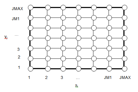
The PDE and BC will be solved using a finite difference method. A grid point formulation rather than a grid block formulation will be used since the dependent variables are specified at the boundaries rather than their flux or normal derivative. The computation domain will be discretized such that the boundary conditions and dependent variables are evaluated at x₁,x₂,…,x_JM1,x_JMAX and y₁,y₂,…,y_JM1,y_JMAX. The finite difference grid appears as follows.

Figure 11.1. 

Finite difference grid for discretizing PDE (grid point formulation)

The unit square is now discretized into JMAX by JMAX grid points where the boundary conditions and dependent variables will be evaluated. The grid spacing is δ=1/(JMAX–1). The first and last row and column are boundary values.

The partial derivatives will be approximated by finite differences. For example, the second derivative of vorticity is discretized by a Taylor's series.

(11.8)

The finite difference approximation to the PDE at the interior points results in the following set of equations.

(11.9)

The vorticity at the boundary is discretized and expressed in terms of the components of velocity at the boundary, the stream function values on the boundary and a stream function value in the interior grid. (A greater accuracy is possible by using two interior points.) The stream function at the first interior point (i=2) from the x boundary is written with a Taylor's series as follows.

(11.10)

The choice of sign depends on whether x is increasing or decreasing at the boundary. Similarly, on a y boundary,

(11.11)

The boundary condition on the stream function is specified by the normal component of velocity at the boundaries. Since we have assumed zero normal component of velocity, the stream function is a constant on the boundary, which we specify to be zero.

The stream function at the boundary is calculated from the normal component of velocity by numerical integration using the trapezodial rule, e.g.,

The finite difference equations for the PDE and the boundary conditions are a linear system of equations with two dependent variables. The dependent variables at a x_i, y_j grid point will be represented as a two component vector of dependent variables,

(11.12)

The pair of equations for each grid point can be represented in the following form

(11.13)

Each coefficient is a 2x2 matrix. For example,

(11.14)

The components of the 2x2 coefficient matrix are the coefficients from the difference equations. The first row is coefficients for the stream function equation and the second row is coefficients for the vorticity equation. The first column is coefficients for the stream function variable and the second column is the coefficients for the vorticity variable. For example, at interior points not affected by the boundary conditions,

(11.15)

The coefficients for the interior grid points adjacent to a boundary are modified as a result of substitution the boundary value of stream function or the linear equation for the boundary vorticity into the difference equations. The stream function equation is coupled to the vorticity with the e_ij coefficient and the vorticity equation is coupled to the stream function through the boundary conditions. For example, at a x=0 boundary, the coefficients will be modified as follows.

(11.16)

If the boundary condition is that of zero vorticity as on a surface of symmetry, it is necessary to only set to zero the coefficient that multiplies the boundary value of vorticity, i.e.,

The linear system of equations and unknowns can be written in matrix form by ordering the equations with the i index changing the fastest, i.e., i=2,3,…,JMAX–1. The linear system of equations can now be expressed in matrix notation as follows.

(11.17)

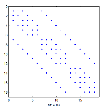
The non-zero coefficients of coefficient matrix A for JMAX=5 is illustrated below. Since the first and last grid points of each row and column of grid points are boundary conditions, the number of grid with pairs of unknowns is only 3x3. Only one grid point is isolated from boundaries. The i,j location of the coefficients become clearer if a box is drawn to enclose each 2x2 coefficient.

Figure 11.2. 

Most of the elements of the coefficient matrix are zero. In fact, the coefficient matrix is a block pentadiagonal sparse matrix and only the nonzero coefficients need to be stored and processed for solving the linear system of equations. The non-zero coefficients of the coefficient matrix are stored with the row-indexed sparse storage mode and the linear system of equations is solved by preconditioned biconjugate gradient method (Numerical Recipes, 1992).

The row-indexed sparse matrix mode requires storing the nonzero coefficients in the array, sa(k), and the column number of the coefficient in the coefficient matrix in the array, ija(k), where k=1,2,…. The indices that are needed to identify the coefficients are the i,j grid location (i,j=2,3,…,JMAX–1), the m equation and dependent variable identifier (m=1 for stream function; =2 for vorticity), and the IA row index of the coefficient matrix (IA=1,2,3,4,…,2(JMAX–2)2). The coefficient matrix has two equations for each grid point, the first for the stream function and the second for vorticity. The total number of equations is NN=2(JMAX–2)2.

The diagonal elements of the coefficient array are first stored in the sa(k) array. The first element of ija(k), ija(1)=NN+2 and can be used to determine the size of the coefficient matrix. The algorithm then cycles over the pairs of rows in the coefficient matrix while keeping track of the i,j locations of the grid point and cycling over equation . The off-diagonal coefficients are stored in sa(k) and the column number in the coefficient matrix stored in ija(k). As each row is completed, the k index for the next row is stored in the first NN elements of ija.

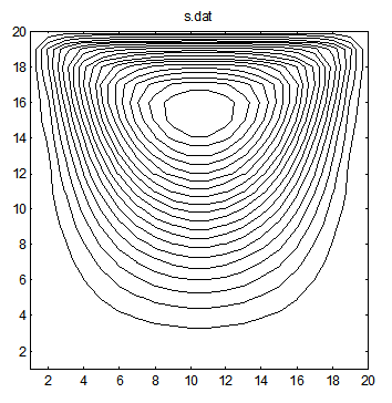
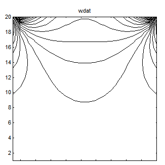
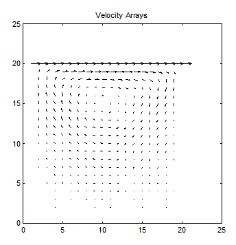
A test problem for this code is a square box that has one side sliding as to impart a unit tangential component of velocity along this side. All other walls are stationary. The stream function, vorticity, and velocity contours for this problem with a 20x20 grid is illustrated below.

Figure 11.3. 

Stream function contours for square with top side sliding

Figure 11.4. 

Figure 11.5. 

Velocity vectors for square with top side sliding

Use the code in the /numer/ directory of the CENG501 web site as a starting point. Add the capability to include arbitrarily specified normal component of velocity at the boundaries. The stream function at the boundary should be numerically calculated from the specified velocity at the boundary. Test the code with Couette and Plane-Poiseuille flows first in the x and then in the y directions. Display vector plot of velocity and contour plots of stream function and vorticity. Show your analysis and code.

Form teams of two or three and do one of the following additions to the code. Find suitable problems to test code.

Form new teams of two or three with one member that developed each part of the code. Include all features into the code. Test the combined features. Work together as a team to do the following simulation assignments.

Boundary layer on flat plate. Compute boundary layer velocity profiles and drag coefficient and compare with the Blasius solution. What assumption is made about the value of the Reynolds in the Blasius solution?

Flow around cylinder. Assume potential flow far from the cylinder. Calculate drag coefficient as a function of Reynolds number and compare with literature.

Flow around cylinder. Find the Reynolds number at which boundary layer separation occurs.

Modern FORTRAN compilers in the MSWindows are very user friendly. They have built in project workspace routines, documentation, and integrated editor and debugger. If you use the FORTRAN compiler on Owlnet, it is useful to know how to use make files to compile and link FORTRAN code. The following is an example make file. You may give it the name, makefile, with no extension.

f77 -c streamf1.f;
f77 -c bc1.f;
f77 -c coef1.f;
f77 -c asolve.f;
f77 -c atimes.f;
f77 -c dsprsax.f;
f77 -c dsprstx.f;
f77 -c linbcg.f;
f77 -c snrm.f;
f77 -o exe streamf1.o bc1.o coef1.o asolve.o atimes.o dsprsax.o dsprstx.o linbcg.o snrm.o

You have to give yourself permission to execute the make file with the one-time command,

chmod +x makefile

The line with the -c option compiles the source code and makes an object code file with the extension of .o. The line with the -o option links the object files into the executable file called exe. This executable file can be executed by typing its name, exe, on the command line.

This example makefile is not very efficient because it will compile every source code listed. There are instructions to recompile only the source code that has been modified or "touched" since the last time the makefile was invoked. However, I do not recall the instructions.

If you are not familiar with FORTRAN, you should get a paperback book on FORTRAN-77 or FORTRAN-90. An example is D. M. Etter, Structured FORTRAN 77 for Engineers and Scientists. The following is a tutorial from the CAAM 211 webpage. http://www.caam.rice.edu/ caam211/JZoss/project1.html

Computer facilities that have compilers usually have an interactive debugger. However, I have not found how to access the debugger on owlnet. The debugger with the Microsoft FORTRAN Powerstation (now HP FORTRAN) is very easy to use.

The development of numerical simulators should start with a problem for which exact solutions exist so that the numerical algorithm can be verified. Steady, creeping flow has many exact solutions and thus it was used as the starting point for developing a numerical simulator for the Navier-Stokes equations. The student should verify that their code is able to duplicate exact solutions to any desired degree of accuracy.

The next stage in the development of the code is to add transients and finite Reynolds numbers. Finite Reynolds number results in nonlinear terms in the Navier-Stokes equation. Algorithms for solving linear systems of equations such as the conjugate gradient methods solves linear systems in one call to the routine. Nonlinear terms need to be iterated or lagged during the transient solution. Thus nonlinear steady state flow may be solved as the evolution of a transient solution from initial conditions to steady state.

The transient and nonlinear terms now need to be included when making the vorticity equation dimensionless.

(11.18)

Two of the dimensionless groups can be set to unity by expressing the reference time in terms of the ratio of the characteristic velocity and characteristic length. The remaining dimensionless group is the Reynolds number.

(11.19)

The dimensionless equation for vorticity with the * dropped is

(11.20)

The convective derivative can be written in conservative form by use of the continuity equation.

(11.21)

We will first illustrate how to compute the transient, linear problem before tackling the nonlinear terms. Stability of the transient finite difference equations is greatly improved if the spatial differenc