Analysis of macroscopic systems usually assume the fluid-fluid interface to simply be a surface of discontinuity in the density and viscosity of the bulk phases with no discontinuity in stress, (i.e., continuous pressure and shear stress across the surface). If there is no significant mass transfer, the surface is also a material surface and thus follows the motion of the fluid particles at the surface.

Systems with a length scale about a centimeter or less and having fluid-fluid interfaces can no longer neglect the discontinuity in stress across the interface. A momentum balance across the interface is needed to describe the stress at the boundary. Also, if the system has surface-active components that affect the surface tension and/or surface viscosity, then a material balance is also needed to determine the composition of the interfacial region. A general treatment of the momentum balance at fluid-fluid interfaces is given in Chapter 10 of Aris, Vectors, Tensors and the Basic Equations of Fluid Mechanics. We summarize the results here assuming no slip at the surface and a Newtonian surface constitutive relation. The terms in the momentum balance are given on the left side and its description is given on the right side.

The surface constitutive equation for a Newtonian interface is (Slattery, 1990)

T ^s = [ σ + ( κ + ε ) ∇_s • v ^s ] I ^s + 2 ε e_s

The surface properties are a function of the composition of the interface. The species mass balance at the interface is given as (Edwards, et al., 1991)

(10.1)

The parallel between the mass and momentum balances and constitutive equations for interfaces and bulk fluids should be noted (Gurmeet Singh, 1996). This analogy with bulk fluids is more complete if a surface pressure due to the reduction of the surface or interfacial tension due to adsorption is defined.

The surface properties are as follows.

Table 10.1.

Symbol	Property
γ	mass per unit area
Γn	surface excess concentration of species n
σ	surface or interfacial tension
π	surface pressure
κ	surface dilatational viscosity
ε	surface shear viscosity
	surface tensors
εαβ	surface permutation symbol
	surface velocity
jns	surface diffusional flux
H	mean curvature
K	Gaussian or total curvature

The normal component of stress. The discontinuity in the normal component of the total stress tensor for a hydrostatic system is as follows.

(10.3)

where H is the mean curvature of the surface and σ is the surface or interfacial tension. The mean curvature can be expressed as a function greatest and least curvatures of curves in the surface k₁ and k₂ or the principal curvatures in the directions of the principal curvature.

The curvature in one of the principal directions can be expressed in terms of the equation for the arc of the curve. Suppose one principal direction is in the x-y plane.

(10.5)

Thus the curvature can be determined from the coordinates of the surface. We see that when the slope is small, the curvature can be approximated by the second derivative. A surface that is translational symmetric has zero curvature in one direction (e.g., surface of a cylinder). The two principal curvatures are equal on the surface of a sphere. A saddle shaped surface can have zero curvature because the principal curvatures have opposite signs.

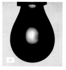
The difference in pressure across a curved interface is called the Laplace pressure after the Laplace-Young equation. This is a classical equation used to determine the shape of a static meniscus or to determine the surface tension from the shape of a static meniscus such as the pendant drop shown here. This is a drop of water suspended from the tip of a capillary tube surrounded by air. Water surrounded by oil would be similar. Suppose we let the origin our coordinate system be the bottom of the drop. The system is an axisymmetric and has two radaii of curvature.

Figure 10.1. 

Pendant water drop in air (Adamson, 1990)

(10.6)

The system is hydrostatic so the pressure profile can be expressed as the pressure jump at the origin and the difference in hydrostatic pressure along the profile.

(10.7)

where Δp_o Laplace pressure at the apex of the drop and r_o is the radius of curvature of the apex of the drop.

The surface or interfacial tension is found using the pendant drop analysis by estimating the value of the tension that best fits the calculated meniscus shape with the shape captured in a video image.

When the pendent drop apparatus is designed so the meniscus is pinned to either the inner or outer edge of the tip of the needle, the contact angle does not influence the shape of the meniscus. If the drop rests on a flat surface, it is called a sessile drop and the elevation of the profile from the surface is a function of the contact angle that the meniscus makes with the substrate.

A characteristic length scale can be determined for the hydrostatic meniscus. Suppose that the datum of elevation corresponds to the apex of the drop. The hydrostatic profile is described by the following dimensionless Young-Laplace equation.

(10.8)

If the dimensionless group is specified to equal unity, a characteristic length is defined.

(10.9)

This characteristic length, called the capillary constant, is sometimes defined with a factor of 2 multiplying the surface tension. It has a value of 2.7 mm for the water-air interface at ambient conditions. This length is representative of the meniscus height of water next to a vertical wall that is wetted by water.

The dimensionless differential equations are now as follows.

(10.10)

(10.11)

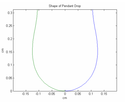
The system of ODEs is computed from the apex of the drop where the dimensionless radius of curvature at the apex is a parameter, B. The value of B is adjusted until the best fit of the measured drop shape is obtained.

Estimation of surface tension. Estimate the surface tension of a dilute surfactant solution, given the shape of a pendant drop shown here and data stored in the file, shape.dat in the Surface directory. You may use the code in pendant.m in the Surface directory to generate the dimensionless pendant drop profiles. Use units.m to plot the drop shape. Note: The program is not automated. Pendant.m computes the dimensionless shape and units.m converts it to cgs units to compare with the measured profile.

Figure 10.2. 

Surface tension gradients. If the system has only two components, i.e., the components comprising each phase then the surface or interfacial tension and contact angle is all that is required to describe the surface effects. However, if the system has another component that is surface active as to adsorb at the interface and reduce the surface or interfacial tension, then the interface must be treated as a two dimensional phase for which a mass and momentum balance is required. The mass per unit area of the surface-active component is the surface excess concentration or the amount adsorbed. If the system is not at equilibrium, i.e., not hydrostatic, then concentration gradients may exist in the interface that result in surface tension gradients in the interface. The difference between the clean interface tension and the local tension is called the surface pressure. The gradients in the surface pressure contribute to tangential stresses in the interface. It has the same role in the surface momentum balance as pressure gradient in the momentum balance for three-dimensional flow. For example, as liquid drains from a soap film, the drag of the liquid on the interface stretches the interface. The resulting expansion of the interface reduces the surface concentration of soap on the interfaces. This establishes a surface tension or surface pressure gradient between the interface in the film and the interface in the meniscus. This gradient tends to oppose the motion of the interface and thus tends to maintain the interface immobile as the liquid drains from between the two near-immobile interfaces. At the same time this surface tension gradient tends to pull the interface from the meniscus back into the film. This leads to a turbulent motion of the interface at the boundary between the meniscus and the film. This effect called "marginal regeneration" is a Marangoni effect caused by the surface tension gradient.

Figure 10.3. 

Plate IV. An irregular mobile film in a vertical rectangle

Figure 10.4. 

Plate I. Rigid film in a rectangular vertical

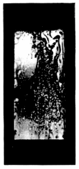
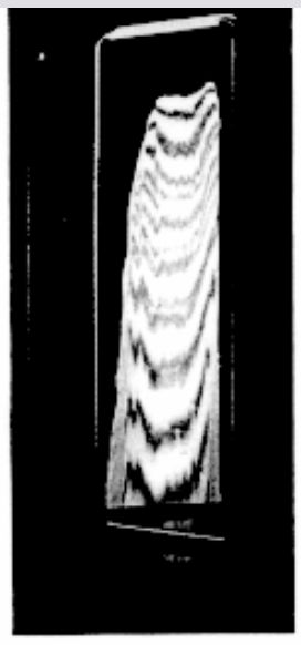
Surface viscosity. Adsorption of a surface-active component at an interface not only changes the surface tension or surface pressure but can also affect the surface rheology. Material adsorbed at interfaces form two-dimensional surface phases that may be gasous, expanded liquid, condensed liquid, or solid. The surface viscosity can change by more than a order of magnitude at a transition from one surface phase to another. This is analogous to the change in viscosity of bulk fluids at phase transitions. The attached figure shows vertical soap film drainage of a system is similar to that of the mobile film except that dodecanol was added to the sodium dodecyl sulfate (SDS) solution. The dodecanol screens the electrostatic repulsion of the SDS at the interface and promote the formation of a condensed liquid monolayer. This monolayer is rigid in this system and the films drains much more slowly than in the case of the mobile film. The mechanism of this difference in the drainage of foam films has been explained in terms of the surface tension gradient driven instability and the stabilizing effect of a large surface viscosity (Joye, et al., 1994, 1996).

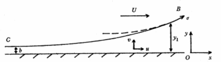
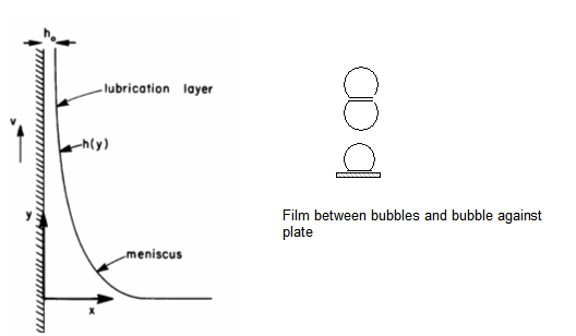
In Chapter 8 we modeled the gravity drainage of a film along a wall neglecting the pressure between the liquid and gas because the mean curvature of the system was very small compared to the length of the film. Now suppose that we have a film that in connected to a curved meniscus. The meniscus may be moving along a substrate and depositing a film or gathering up a deposited film, e.g., a bubble in a capillary tube. Alternatively, the substrate may be stationary with respect to the meniscus and the film is draining into the mensicus, e.g. foam or emulsion film between two bubbles or drops. For simplicity, we will assume that we have a pure system so there are no surface tension gradients or effects of surface viscosity. We will assume that the system is translational invarient. A schematic of some possible system configurations are shown below.

Figure 10.5. 

Section of a bubble in a horizontal tube.

Figure 10.6. 

The transition region.

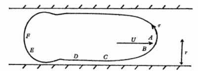
Configration of a bubble in a tube (Breatherton, 1961)

Figure 10.7. 

The continuity equation and equations of motion were specialized for lubrication and film flow in Chapter 6. The equations to or are as follows.

(10.12)

The systems with a solid substrate will have the boundary condition of no-slip at the solid boundary and zero shear stress at the pure-fluid interface. In the case of two bubbles or drops coming into contact, the mid-plane is a plane of symmetry and has zero shear stress. It will be assumed the fluid interface is immobile in this latter case. The variable, h, is the half-film thickness in this case. Since this case has zero shear on one surface and no slip on the other surface, the solution will be derived as for the cases with the solid substrate. The boundary conditions are as follows.

(10.13)

The pressure is uniform across the thickness of the film so the velocity profile can be determined by integrating the equation of motion over the film thickness and applying the boundary conditions.

(10.14)

The average velocity is substituted into the equation of continuity.

(10.15)

The pressure can be expressed in terms of the thickness by application of the Young-Laplace equation assuming that the system has no dependence on x₂.