Chapter Three
3. SIMULATING MEMBRANE PROTEINS
Nilay K. Roy *
ITS-Research Computing, Northeastern University,
360 Huntington Avenue, Boston, MA 02115, USA
ABSTRACT
Membrane proteins may contain a significant portion of their mass within the interior of the membrane or are only associated to the membrane surface. The transmembrane (TM) part can be -helical or have a -sheet topology. The TM part can have a variety of sizes, molecular weights and conformations. Membrane proteins govern biological processes such as energy conversion, transport, signal recognition and transduction. Up to 30% of the encoded proteins in the genome of all organisms are such proteins, and they are 60% of all drug targets. Currently less than 1% of the protein structures deposited in the RCSB Protein Data Bank are membrane proteins. Simulating membrane proteins provides an alternative way to study them. Ion channels are a class of membrane proteins where passive transport is influenced by the membrane potentials. Many such ion channels have a selectivity filter and a gating mechanism embedded in the membrane core. Asymmetric ion concentrations across the membrane also affect transport and protein functions. These are difficult to study. Large scale molecular dynamics (MD) with coarse graining in both the membrane lipid bilayer and in parts of the membrane protein itself is generally the method used in any simulation study to understand the mechanisms of such proteins' structure-function relationships and dynamic modes. Principal component analysis of the protein is also frequently used. This chapter gives an overview of the current simulation methods used to prepare and study membrane proteins. The focus is on large scale simulations with special emphasis on scalable parallel methods. Correctly relating molecular structures to the physiological properties of the protein is a major challenge in the field. All the effects of the inhomogeneous lipid bilayer, potentials, ion/anion concentrations, that cover both spatial and temporal scales must be included. This has challenges when systems have thousands of explicit atoms and require simulations on the micro-second scale. We review these challenges and explain methods that have been used to overcome the shortcomings of explicit MD simulations.
Keywords: membrane proteins, transmembrane, genome, molecular dynamics, ion/cation concentrations, membrane potentials, force fields, semi-explicit methods, lipid, membrane curvature
* Current affiliation: The Charles Stark Draper Laboratory, Inc. (Draper), 555 Technology Square, Cambridge, MA 02139-3563. Tel:(617)258-1515. E-mail: nroy@draper.com.
3.1. INTRODUCTION
Molecular dynamics (MD) simulation is a molecular mechanics approach that is implemented using numerical methods that study the motion of a system of particles (atoms, molecules, entities) under the influence of internal and external forces (Chandler, 1987). These forces are interactions between the particles, which are influenced by other parameters such as temperature, pressure, and additional constraints (Lindahl, Hess and van der Spoel, 2001). Additional constraints include forces in steered or targeted MD. The empirical potential energy function that relates structure to energy and describes the forces between atoms using harmonic and periodic potentials to model covalent bond mediated interactions, as well as Coulomb and Lennard Jones-like potentials to represent electrostatic and van der Waals interactions, form the basis of MD force calcuations (MacKerell, 1998). These forces are called “force fields”. Typically calculated in a few femtosecond time steps they predict how each atom will move. Repeating the time step millions of times, a trajectory of all atoms in the system over time is generated that permits studying the dynamics of the (membrane) protein of interest and its microenvironment at a level of detail not accessible by laboratory experiments (Stansfeld and Sansom, 2011; Ingólfsson et al., 2016). By parallelizing the system using a large cluster of computers it is now possible to simulate a range of system sizes up to several million atoms even on a millisecond time scale (Allen et al., 2001; Rapaport, 2004; Klepeis et al., 2009). Several force fields have been developed like AMBER, CHARMM, and GROMOS (Patel et al., 2004; Case et al., 2005; Christen et al., 2005). Typically in MD simulations of very large explicit systems, it is well known that there are several problems. These include exponentially increasing equilibrium and non-equilibrium relaxation times, correlation times and lengths (Stanley, 1971). In very large systems there are problems like critical slowing down and other finite size effects that can take on special significance (Ceriotti, Bussi and Parrinello, 2010). Furthermore, with any simulation the full characterization must have reliable error estimates. This can only be obtained after several runs from a number of different initial starting configurations. Figure 1 gives an example of time and length scales of different computational methods. In any MD system considerations must also include the ensemble to be used – for example NVE (micro-canonical), NPT or NVT (Leach, 1996). An important consideration here is if diffusion is needed. Then the density varies, and a grand-canonical enbsemble may be more favorable over the canonical NPT (Frenkel and Smit, 1996). NPT is generally also preferable if you want to equilibrate the system. NVT is then used to collect statistics of interest.
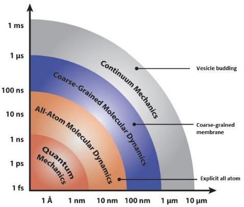
Figure 1. Computational methods over a range of length and time scales in membrane protein simulations.
Another important consideration is creating the starting structures and system of MD simulations. The membrane protein environment is characterized by two different chemical regions that have to be modelled correctly by the force field (Allen and Tildesley, 1987). This is done using implicit or explicit representations of the lipid and water phases. In general if the reported protein structure is used there are many defects. These include overlapping atoms, missing hydrogens, improper N and C terminus and so on. If modeled the total energy of the system would explode. The entire protein with the lipid membrane, water, and ion/counterions has to be systematically relaxed, overlapped and equilibrated. For water soluble proteins, generation of the initial system is completed by solvating the system with a water/ion solution (Marrink, Devries and Tieleman, 2009). However, membrane protein simulations require the additional working step of accommodating the protein in the bilayer. Here either the bilayer is constructed around the protein, or the protein is inserted into a pre-equilibrated bilayer. As shown in Figure 2 there are a number of tranmembrane protein toplogies.
Depending on the protein’s shape, its cavity structure in the trans-membrane section, the number of membranes spanned by the protein and the membrane curvature (plane bilayer versus vesicles or micelles), individual challenges arise that have to be taken into account by both accommodation strategies (Van der Ploeg and Berendsen, 1983). Table 1 gives the times and sizes of some MD simulations of membranes (Stansfeld, Jefferys and Sansom, 2013; Chavent et al., 2015; Koldsø and Sansom, 2015; Reddy et al., 2015). These larger scale models also enable studies of the collective behaviour of multiple copies of membrane proteins, such as the influence of crowding of membrane proteins on their clustering and diffusion (Janosi et al., 2012; Chavent et al., 2014). The dynamic properties of membranes play a key role as regulatory mechanisms and will influence the mechanical properties of cell membranes.
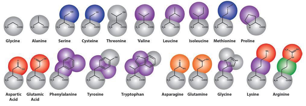
Figure 2. Martini coarse-grained model extension to amino acids, colored by bead type (where purple is apolar, blue and green are intermediate, gray and orange are polar and red represents charged particles).
Table 1. For each MD system, the granularity of the simulation (atomistic versus coarse-grained), the number of atoms/particles (including water) in the simulation system, the duration of the production run simulation, the approximate linear dimension of the simulation box, and the resultant trajectory file size are given.
3.2. COARSE GRAINED MD SIMULATIONS
In coarse grained models the length-scale at which chemical components are modeled become important. Such a model necessarily lumps many atomic degrees of freedom into a single coarse-grained bead. As with the MD approach the coarse grained molecular model (CGMD) treats molecules classically. Newton’s laws of motion are integrated according to potentials, which define the forces beween each bead in the system.

Eq 1 describes the motion of N particles, each with mass, mi, experiencing a force, Fi, due to a potential energy function, V, itself a function of the configuration of all atoms in the system that are close enough to exert a measurable force. NAMD (Phillips et al., 2005) integrators is one software package that can be used for CGMD to perform simulations. MD simulations make contact with observables, like temperature and pressure. Temperature is defined by the kinetic energy of the particles, while macroscopic pressure is defined by the average of the molecular virial given in Eq 2 and Eq 3, respectively.
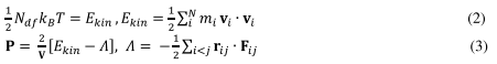
V is the volume of the system, Ekin is the kinetic energy, rij is the distance vector between particles, i and j, Fij is the corresponding force, Ndf is the number of degrees of freedom (3N - 3 for N particles, minus any constraints) and is the virial. The choice of these forces and the physical quantities they representdispersion forces, electrostatics and bonded forces-define themodel and determine its ability to reproduce observed physical phenomena. CGMD can be done on models built using structure-based, force-based and energy-based force-fields. Because coarse-graining requires a simplification of many degrees of freedom, it is impossible to build a model that simultaneously reproduces all of the geometric, thermodynamic and kinetics features of a physical system. To build a coarsegrained model, it is therefore necessary to choose which physical properties are essential to the behavior of the target system. Examples of such systems are reviewed extensively (Shelley et al., 2001; Izvekov and Voth, 2005; Ayton and Voth, 2009; Shinoda, DeVane and Klein, 2010).
In the “Center for Molecular Modeling Coarse-Grained” (CMM-CG) (Shinoda, DeVane and Klein, 2010) model the entire structural properties of the dimyristoylphosphatidylcholine (DMPC) bilayer is reproduced. The CMM-CG model maps three water molecules onto a single bead. Non-bonded forces are modeled with general Lennard-Jones (LJ) potentials with a potential well depth and zero-position, which is tuned to reproduce the desired structure and thermodynamic properties of the target system. The softer 12-4 potential is used to model dispersion forces in water by matching the melting temperature, density and vapor pressure observed in bulk and thin-film test simulations. A potential of mean force (PMF) between CG beads is then estimated using pair correlation functions, or radial distribution functions (RDF).
In the case of “Force Matching with the Multiscale Coarse Grained” (MSCG) (Ayton and Voth, 2009) model, force-matching to develop a rigorous coarsegrained force field directly from forces measured in all-atom simulations was used. A variational method in which a coarse-grained force field is systematically developed from all-atom simulations under the correct thermodynamic ensemble. It is now possible to develop the exact many-body coarse-grained PMF from a trajectory of atomistic forces with a sufficiently detailed basis function.
Introducing protein detail to a coarse-grained force field requires an accurate model for both of the structure and dynamics of the protein itself, as well as the interactions with surrounding lipids and solvent. One example of such coarse graining is in the so called “Martini Proteins” (Marrink, de Vries and Mark, 2004). In the Martini force field, amino acids are mapped onto as many as five beads (Figure 2), one of which represents the polypeptide backbone. Residues with rings (His, Phe, Tyr, Trp) use a finer mapping and improper dihedral terms to preserve the topology of these rings. Intra-amino acid bonded potentials, angles and dihedrals have equilibrium values equal to the average of distributions measured from all bonded amino acid pairs found. These are sorted by helix, coil and extended secondary structure, as measured by the DSSP (“define secondary structure of proteins”) prediction algorithm (Kabsch and Sander, 1983), so that the Martini model includes the effect of secondary structure on the apparent hydrophobicity and polarity of its constituent particles. This secondary structure remains fixed throughout the simulation. Thus the Martini model cannot sample secondary structure changes. It is possible to reconstitute atomistic details from a coarse-grained simulation using a “back-mapping” procedure similar to simulated annealing (Rzepiela et al., 2010). By tuning these models it is possible for CGMD to accurately explain protein-bilayer interactions, peptide self-assembly and protein binding. These methods can also model internal structural changes that guide the biological functions of many proteins.
3.3. ASYMMETRIC ION CONCENTRATIONS
Differences in ion concentrations across the membrane that are established under the action of various membrane transport proteins can give rise to a difference in electric potential. Reproducing this set of conditions in computer simulations is not trivial. Several methods have been used successfully to simulate this effect. To allow for the simulation of ion channels with a realistic implementation of asymmetric ion concentration and transmembrane potential boundary conditions, a grand canonical Monte Carlo (GCMC)/Brownian dynamics (BD) was implemented in one case (Lee et al., 2012). Here asymmetric boundary conditions were imposed on a finite nonperiodic simulated system surrounded by concentration buffer regions. Insight into the factors governing the permeation of wide aqueous pores was possible. Imposing asymmetric concentrations in explicit solvent MD is difficult. Such explicit solvent MD simulations are normally performed with conventional periodic boundary conditions (PBCs), which are critical to reduce finite-size effects. Unavoidably, the PBCs also eliminate the distinction between the two sides of a membrane. Because there is a single continuous bulk solution where ions are free to diffuse and equilibrate, concentration gradients across the membrane cannot be simulated. To overcome this simulation of asymmetric ion concentrations in MD simulations with explicit solvent using a dual-membranes–dual-volumes strategy was tried (Delemotte et al., 2011). Two spatially separated membranes are included to create two disconnected bulk phases between them. In a more recent effort one of the two membranes is replaced by an artificial vacuum separator to reduce the computational burden (Delemotte et al., 2008). In another case manually adjusting the number of cations and anions in the two bulk regions makes it possible to set the effective membrane potential near some pre-chosen value Vm (Kutzner et al., 2011). These methods serve to increase computational costs. Other attempts include introducing energy steps at the boundaries of the periodic cells that separates the two solutions and generates a nonuniform distribution of the solute molecules across the cell boundaries with assymetric external fields. These result in a net charge imbalance across the membrane (Gumbart et al., 2012). There is no simple relationship between the energy step, the charge imbalance, and the resulting membrane potential.
3.4. INTERFACE OF MEMBRANES
One interesting set of problems concerns the mechanism by which small peptides and peripherally associated membrane proteins bind to and interact with the water/membrane interface. Studies include membrane lytic toxins, model peptides, fusion proteins, and peripherally associated signal transduction proteins and biosynthetic enzymes. For example in one study (Huang et al., 2003) implicit solvent calculations were used on cobra cardiotoxin CTX A3 to interpret polarized attenuated total internal reflection infrared spectroscopy data, suggesting modes of binding of this toxin to zwitterionic and anionic membranes. This toxin appeared to have a greater thinning effect on anionic phosphatidylglycerol monolayers than on those composed of zwitterionic phosphatidylcholine species.
A number of other membrane–water interface associated peptides have been investigated. One study used the HIV fusion protein gp41 and mutants in POPE bilayers (Wong, 2003), with comparison between simulations and attenuated total internal reflection infrared spectroscopy to determine the orientation of peptides relative to the bilayer. The simulation component of this study involved the removal of several lipids from one leaflet in order to accommodate protein inclusion.
Several larger peripheral membrane proteins have been investigated by MD. One study looked at cytochrome c in association with different alkanethiol selfassembled monolayers, with the aim of understanding the structural features of the protein in these complexes and the nature of the monolayer association. Many peripherally associated proteins have important roles in signal transduction and disease, and simulations continue to be a powerful method to understand the detailed lipid–protein interactions responsible for their activity.
Figure 3 shows an example of the membrane anchored protein prostaglandin H2-synthase. Its substrate, arachidonic acid, is a fatty acid in the membrane and cannot be found in the cytoplasm. The only way to effectively study such a protein is by using large scale simulations.
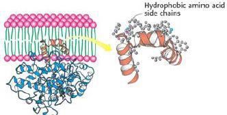
Figure 3. The membrane-anchored protein prostaglandin H2-synthase.
Figure 4 shows an example of hydration of the head group region in both coarse-grained (A) and all-atom models (B) of a membrane (lipids are removed). After large scale MD simulations reverse coarse-graining is done mapping back coarse-grained beads to the all-atom clusters, and resolvating the system. Minimization steps with simulated annealing while constraining atoms to the postion of the corresponding coarse-grained beads completes the process.
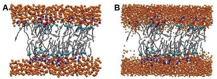
Figure 4. Hydration of the heads group region in both coarse-grained (A) and allatom models (B) of a membrane protein. Lipids are removed.
3.5. TRANSMEMBRANE SIMULATIONS
It is known that membrane spanning helices can be considered the smallest autonomous membrane protein domains. Simulations can be done in order to study the properties of fundamental interest, such as the dynamics of isolated helices (Bright and Sansom, 2003), protein–lipid interactions (Petrache et al., 2002), helix association (Stockner et al., 2004), and the behaviour of simple channels such as those formed by certain fungal proteins and toxins (Tieleman and Sansom, 2001). MD simulations have also looked at the effects of hydrophobic mismatch on peptide and bilayer dynamics. Mismatch results when the effective hydrophobic thickness of the bilayer does not match that of a perfectly transmembrane-oriented helix (de Planque and Killian, 2003). Several mechanisms might compensate for this mismatch, including changes in peptide tilt, changes in secondary structure, peptide association, aggregation of different lipid species near the protein, and adaptation of bilayer structural properties like thickness or curvature. The dynamic properties of individual helices can be examined in detail with MD. A number of proline and glycine-containing sequence motifs have been extensively studied. Transmembrane helix flexibility mediated by specific sequence motifs have important consequences for the activity of membrane proteins such as gated ion channels (Capener and Sansom, 2002; Treptow, Marrink and Tarek, 2008; Nishizawa and Nishizawa, 2009; Delemotte et al., 2010; Khalili-Araghi et al., 2012; Li and Gong, 2015). The number of transmembrane helices in membrane proteins ranges from 1 to 14. A single transmembrane helix in bitopic membrane proteins are the most numerous. The second most numerous membrane proteins are those with seven transmembrane helices (Crozier et al., 2003), followed by proteins with 2, 4 and 12 transmembrane helices.
The dynamic properties of individual helices can be examined in detail with MD. Ion-channel pore helices like proline-kinked helices have been extensively studied. Proline and glycine are both thought to be important mediators of hingebending motions. Proline disrupts normal helical hydrogen bonding and participates in repulsive steric interactions with adjacent backbone atoms. A study on TMH-2 of the chemokine receptors identified a highly conserved TXP sequence motif by multiple sequence alignment (Govaerts et al., 2001). MD simulations were employed to investigate the effects of this sequence on the behavior of polyalanine in a hydrophobic environment. This indicated that the hydroxyl-containing amino acids also modulate the kink behavior of prolinecontaining sequences.
The interaction between α-helices is thought to be one of the most important determinants of membrane protein structure and function (Olivella et al., 2002). Proteins comprising pairs of α-helices can be employed as models for understanding these interactions. To get the interactions between pairs of helices simulated annealing and global searching MD (Kochva, Leonov and Arkin, 2003) or Monte-Carlo simulations (Kessel et al., 2003), either with an all-atom MD force field (Choma et al., 2001) or a simplified interaction potential function (Fleishman and Ben-Tal, 2002) is done.
Proton transport presents a special challenge to MD simulations because protons move between different water molecules and are not easily treated by a classical potential function. Viral and other small ion channels from small proteins (60-120 amino acids) are many such membrane proteins that have proton transport. Gramicidin A (Yu, Cukierman and Pomes, 2003), the influenza A M2 channel (Forrest, Tieleman and Sansom, 1999), and the engineered LS2 channel are examples. Different approaches have been developed for studying proton transport in membrane proteins. One method involves using the PM6 water model. PM6 is a polarizable and dissociable empirical water model consisting of O2- and H+ units (Yu and Pomes, 2003). The empirical valence bond (EVB) theory has also been used to model the LS2 channel (Warshel, 2002). In all cases extensive MD simulations of a multitude of parameters and potential models are done to determine the best fit to experimental observations. These are all areas in which large-scale MD simulations do not provide correct answers.
Another area where explicit MD simulations need to be modified is in the proton exclusion problem, as seen in aquaporins (AQP). These membrane proteins allow water and glycerol to diffuse through while excluding protons, which would otherwise destroy the proton electrochemical gradient and starve cells to death. Several models for proton exclusion have been proposed (Zhu, Tajkhorshid and Schulten, 2001; deGroot et al., 2003; Ilan et al., 2004; Phongphanphanee, Yoshida and Hirata, 2008; Tani et al., 2009) and used with classical and steered (targeted) MD simulations. In simulations looking at water permeation, key structural features including the NPA motif, a constriction region (also termed ar/R), and the helix dipoles have been identified as contributors to this specificity. Methods to quantify water conduction properties such as osmotic permeability of AQP via MD simulation methods have also been developed. These methods involve inducing a hydrostatic pressure difference across a membrane with embedded AQP (Zhu, Tajkhorshid and Schulten, 2004).
In the case of mechanosensitive transmembrane channels (Perozo and Rees, 2003) a combination of MD simulations with normal mode analysis has been successfully used (Bilston and Mylvaganam, 2002; Anishkin et al., 2003; Valadie et al., 2003). However, such simulations typically provide more than one mechanism for opening and closing. These multiple pathways provide a challenge in the absence of crystal structures on either the open or closed states for guidance. High-resolution structural methods cannot access these states. The crystal structures obtained of such states will most likely be a mutant one based on modeling. Figure 5 shows the two open states of the mechanosensitive ion channel MscL (Perozo et al., 2002).
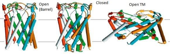
Figure 5. Two possible open states of the mechanosensitive ion channel MscL. MD simulations can predict both types of gating where the pore diameter of one open state (Barrel ~15 Å) is nearly half that of the other (Open TM pore diameter ~ 30 Å).
Direct MD simulations however are shown to be very effective in the case of ABC-type transporters (Higgins, 1992). As one of the largest superfamilies of proteins (Hopfner et al., 2000) ABC-transporters are involved in multidrug resistance in cancer cells and bacteria and in genetic diseases such as cystic fibrosis. They are present in eukaryotic and prokaryotic systems and have the characteristic LSGGQ signature motif in their ATPase domain. Using targeted MD (TMD) it has also been shown how MD can be used for structural modeling. The first reported crystal structure of a “complete” ABC-transporter, MsbA from E. coli (ECMsbA), was resolved at 4.5Å (Chang, 2003). This structure revealed only the C-α polypeptide trace of the protein, and coordinates for a significant part of the nucleotide binding domain (NBD) consisting of 78 residues including the conserved ATP binding “Walker A” motif could also not be determined due to disorder. Starting from the C-α polypeptide trace, the backbone and side chain atoms were generated, and the structure of the missing part of the NBD was modeled based on homology with known high-resolution structures of the NBDs of other ABC transporters. MD simulations were subsequently used to test the stability of the model. While the monomer was stable to MD simulations the dimer was not. In reorienting the transmembrane domains of ECMsbA with respect to the NBDs in order to transform the “back-to-back” dimer into a “headto-tail” model, a suitable template was found to model another ABC-transporter P-glycoprotein (Stenham et al., 2003).
Another avenue used to simulate membrane proteins is biased MD. Using the biasing forces on ATP synthase creates non-equlibrium MD simulations. Steering or acceleration may also be used. This is favored over the regular equilibirum MD. Events of interest like ATP binding or release occur on the millisecond time scale but the large size of the protein limits simulation to the nanosecond. One example is a biasing force to cause 120o rotations of the cental stalk. The drawback with this method is that key relaxation events may be missed when a process that occurs in the millisecond time scale in nature is forced to occur on the nanosecond time scale accessible to protein MD simulations. Biased MD simulations thus do not yield a full transition path. However, useful mechanistic information can still be derived from such studies (Ma et al., 2002).
Finally, processes involving the breaking of chemical bonds cannot be studied using MD. A quantum mechanical (QM) treatment is needed, but QM is computationally expensive and currently limited to a few hundred atoms. The QM/MM (molecular mechanics) method is a technique used to study such systems. The reactive centre and its immediate surroundings are modeled in electronic detail using a quantum mechanical approach while the rest of the system is treated classica