T
V GQ
min
T
V GG Q
4.1 Artificial Neural Network (ANN)
ANN, specifically the MultiLayer Perceptron (MLP), has been successfully used as a
where G is the pseudo inverse of the gain matrix G .
classifier in BCI systems. The units of computation in an ANN is called neuron, in reference
Eq 6 is clearely non linear and would require high computational search in order to find a
to the human neuron it tries to simulate. These neurons are elementary machines that apply
solution. The “MUltiple SIgnal Classification” (MUSIC) has been proposed in (Schmidt
a nonlinear function, generally a sigmoid or a hyperbolic tangent, to a biased linear
1981) to reduce the complexity of this search. The MUSIC algorithm is briefly introduced
combination of its inputs. If xl, …, xl are the neuron input and y is its output, we can write:
hereafter in terms of subspace correlations. Given the rank of the Gain matrix p and the rank
l
(8)
of the signal matrix Fs that is at least equal to p, the smallest subspace correlation value
y f ak x
k
b
represents the minimum subspace correlation between principal vectors in the Gain matrix
k1
and the signal subspace matrix Fs. The subspace of any individual column gi with the signal
where f( ) is the neuron function, b is the bias and { a
subspace will exceed this smallest subspace correlation. While searching the parameters, if
k} are the linear combination weights
representing the synapses connections.
the minimum subspace correlation approaches unity, then all the subspace correlations
In the MLP structure, neurons are organized in layers. The neural units in a layer do not
approach unity. Thus, a search strategy of the parameter set consists in finding p peaks of
interact with each other. They take their inputs from the neurons of the preceding layer and
the metric:
provide their output to the neurons of the next layer. In other words, the outputs of neurons
gT
T
ˆ ˆ
(7)
of layer i-1 excite the neurons of layer i. Therefore, MLP is completely defined by its
2
S S g
subcorr
structure and the connections weights. Once defined, the ANN parameters, the weights for
g
each neuron, must be estimated. This is usually done according to a train set and using the
gradient descent algorithm. In the train set, it is supposed available the inputs and desired
The gain vectors g are considered for all points of a grid that represents the cortical surface.
outputs of the MLP for different experiments. The gradient descent will iteratively adjust the
The point of the grid with the highest subcorrelation coefficient is selected and the algorithm
MLP parameters so as to have its output the closer to the desired output for the different
may tries to have a fine detection of the dipole around this point or restart looking for the
experiments.
next dipole. However, and for the BCI system, the algorithm is stopped at the first stage and
a feature vector is built including all the subspace correlations obtained in the different
points of the grid. This vector is then used as input for the decoding process of the BCI
4.2 Support Vector Machines (SVM)
system.
SVM is a recent class of classification and/or regression techniques based on the statistical
The computation of the subspace correlation coefficients is performed on the points of a grid
learning theory developed in (Vapnik, 1998). Starting from simple ideas on linear separable
representing the cortical surface of the brain. Two grids have been studied: the first, a
classes, the case of linear non-separable classes is studied. The separation of classes using
spherical grid defined to be 1 cm inside the skull; the second, a grid with no analytical form
linear separation functions is extended to the nonlinear case. By projecting the classification
designed to follow, at 1cm distance, the skull. For the nonanalytic grid, the skull has been
problem to a higher dimension space, high performance non-linear classification may be
divided into layers on the z-axis. In every layer, the grid is defined as an ellipse that is 1cm
achieved. In the higher dimension space, linear separation functions are used while the
distant from the skull position. For a few layers, skull points were lacking to precisely define
passage to this space is done with a non-linear function. Kernel functions permit to
the ellipse. In such cases points were borrowed from adjacent layers and a linear
implement this solution without needing the mapping function or the dimension of the
interpolation is performed to estimate the required skull point.
higher space. More detail is provided in (Cristianini & Taylor, 2000). In (Khachab et al., 2007)
The present study uses the MUSIC-like brain imaging techniques of signal subspace
several kernel functions have been used and compared.
correlations and metrics to localize brain activity positions (Mosher & Leahy, 1999). Two
pattern recognition algorithms have been tested as classifiers: the artificial neural network
multilayer perceptron and the support vector machines. Experiments have been conducted
5. Experiments
on subject 1 of a reference database (NIPS 2001 Brain Computer Interface Workshop) (Sajda
5.1 Database
et al., 2003) .
Experiments have been conducted on subject 1 of a reference database from the NIPS 2001
Brain Computer Interface Workshop (Sajda et al., 2003). The “EEG Synchronized Imagined
Movement” database was considered. The task of the subjects was to synchronize an
Brain Imaging and Machine Learning for Brain-Computer Interface
67
where S corresponds to the first p eigenvectors.
4. Classifiers or Decoding Process
Several classifiers have been used in BCI systems. Two principal classifiers are presented
A least square estimation of the current sources consists in minimizing the cost function:
here: Artificial neural network (ANN) and Support Vector Machines (SVM).
2
2
2
(6)
min E min
T
V GQ
min
T
V GG Q
4.1 Artificial Neural Network (ANN)
ANN, specifically the MultiLayer Perceptron (MLP), has been successfully used as a
where G is the pseudo inverse of the gain matrix G .
classifier in BCI systems. The units of computation in an ANN is called neuron, in reference
Eq 6 is clearely non linear and would require high computational search in order to find a
to the human neuron it tries to simulate. These neurons are elementary machines that apply
solution. The “MUltiple SIgnal Classification” (MUSIC) has been proposed in (Schmidt
a nonlinear function, generally a sigmoid or a hyperbolic tangent, to a biased linear
1981) to reduce the complexity of this search. The MUSIC algorithm is briefly introduced
combination of its inputs. If xl, …, xl are the neuron input and y is its output, we can write:
hereafter in terms of subspace correlations. Given the rank of the Gain matrix p and the rank
l
(8)
of the signal matrix Fs that is at least equal to p, the smallest subspace correlation value
y f ak x
k
b
represents the minimum subspace correlation between principal vectors in the Gain matrix
k1
and the signal subspace matrix Fs. The subspace of any individual column gi with the signal
where f( ) is the neuron function, b is the bias and { a
subspace will exceed this smallest subspace correlation. While searching the parameters, if
k} are the linear combination weights
representing the synapses connections.
the minimum subspace correlation approaches unity, then all the subspace correlations
In the MLP structure, neurons are organized in layers. The neural units in a layer do not
approach unity. Thus, a search strategy of the parameter set consists in finding p peaks of
interact with each other. They take their inputs from the neurons of the preceding layer and
the metric:
provide their output to the neurons of the next layer. In other words, the outputs of neurons
gT
T
ˆ ˆ
(7)
of layer i-1 excite the neurons of layer i. Therefore, MLP is completely defined by its
2
S S g
subcorr
structure and the connections weights. Once defined, the ANN parameters, the weights for
g
each neuron, must be estimated. This is usually done according to a train set and using the
gradient descent algorithm. In the train set, it is supposed available the inputs and desired
The gain vectors g are considered for all points of a grid that represents the cortical surface.
outputs of the MLP for different experiments. The gradient descent will iteratively adjust the
The point of the grid with the highest subcorrelation coefficient is selected and the algorithm
MLP parameters so as to have its output the closer to the desired output for the different
may tries to have a fine detection of the dipole around this point or restart looking for the
experiments.
next dipole. However, and for the BCI system, the algorithm is stopped at the first stage and
a feature vector is built including all the subspace correlations obtained in the different
points of the grid. This vector is then used as input for the decoding process of the BCI
4.2 Support Vector Machines (SVM)
system.
SVM is a recent class of classification and/or regression techniques based on the statistical
The computation of the subspace correlation coefficients is performed on the points of a grid
learning theory developed in (Vapnik, 1998). Starting from simple ideas on linear separable
representing the cortical surface of the brain. Two grids have been studied: the first, a
classes, the case of linear non-separable classes is studied. The separation of classes using
spherical grid defined to be 1 cm inside the skull; the second, a grid with no analytical form
linear separation functions is extended to the nonlinear case. By projecting the classification
designed to follow, at 1cm distance, the skull. For the nonanalytic grid, the skull has been
problem to a higher dimension space, high performance non-linear classification may be
divided into layers on the z-axis. In every layer, the grid is defined as an ellipse that is 1cm
achieved. In the higher dimension space, linear separation functions are used while the
distant from the skull position. For a few layers, skull points were lacking to precisely define
passage to this space is done with a non-linear function. Kernel functions permit to
the ellipse. In such cases points were borrowed from adjacent layers and a linear
implement this solution without needing the mapping function or the dimension of the
interpolation is performed to estimate the required skull point.
higher space. More detail is provided in (Cristianini & Taylor, 2000). In (Khachab et al., 2007)
The present study uses the MUSIC-like brain imaging techniques of signal subspace
several kernel functions have been used and compared.
correlations and metrics to localize brain activity positions (Mosher & Leahy, 1999). Two
pattern recognition algorithms have been tested as classifiers: the artificial neural network
multilayer perceptron and the support vector machines. Experiments have been conducted
5. Experiments
on subject 1 of a reference database (NIPS 2001 Brain Computer Interface Workshop) (Sajda
5.1 Database
et al., 2003) .
Experiments have been conducted on subject 1 of a reference database from the NIPS 2001
Brain Computer Interface Workshop (Sajda et al., 2003). The “EEG Synchronized Imagined
Movement” database was considered. The task of the subjects was to synchronize an
68
Biomedical Imaging
indicated response with a highly predictable timed cue. Subjects were trained until their
5.3 Brain Imaging Using MUSIC
responses were within 100 ms of the synchronization signal. Eight classes of trials (explicit
Because the BCI system is based upon the calculation of neural activity on the cortical
or imagined for left/right/both/neither) were randomly performed within a 7 minute 12
surface of the brain, it would be interesting to measure the ability of the MUSIC algorithm to
seconds block. Each block is formed of 72 trials. A trial succession of events is shown in Fig.
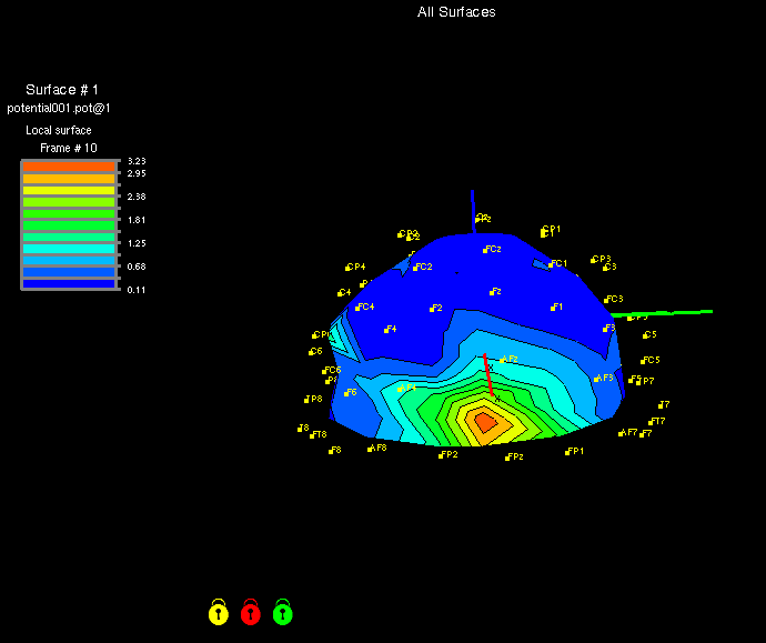
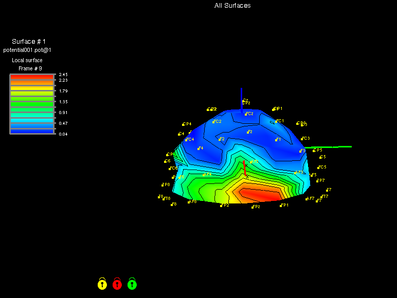
detect this activity. Fig. 7 and Fig. 8 illustrate the subcorrelation coefficients for the 120
6. The EEG was recorded from 59 electrodes placed on a site corresponding to the
points of the non parametric grid in left action and right action. The figures also show the
International 10-20 system and referenced to the left mastoid. In a preprocessing stage,
placement of the skull sensors (International 10-20 system). Figures were obtained using the
artifacts were filtered out from the EEG signals (Ebrahimi et al., 2003), and signals were
MAP3D software. It is clear that electrical activity occurs in the same part of the cortical
sampled at 100 Hz.
surface with deviation depending on the direction of the actions.
One trial – 6 seconds
Trial Event
2 seconds
Blank Screen
500
Fixation
ms
Explicit/Imagined
1
Fixation
second
Fig. 7. Subcorrelation coefficients for left action.
Left/Right/Both/Neither
250ms
1
Fixation
second
X
50ms
Fixation
950 ms
Fig. 6. Illustration of one trial recording (reproduced from
http://liinc.bme.columbia.edu/EEG_DATA/EEGdescription.htm).
Fig. 8. Subcorrelation coefficients for right action.
5.2 Experimental Setup
In order to test the BCI system, we have considered two segments from each period: A
5.4 MLP-Based Classifier
segment of 2 seconds corresponding to the blank screen, and a segment corresponding to
The first set of experiments aimed to optimize the classifier complexity, the number of cells
the thinking of a movement. Only subject 1 was used in our experiments, for whom sensors
in the hidden layer of the ANN. The analysis window on which the MUSIC algorithm is
coordinates (skull) were available. Ninety periods were available for this subject in the
applied had a duration of 640 ms. It was assumed that the space dimension (number of
database. These were divided into 60 periods for training and 30 periods for testing. The
dipoles) is equal to 10. The spherical grid was used in these experiments. The optimal
cortical surface geometrical information was not available, however. Thus, two models have
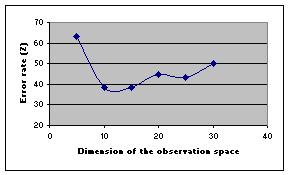
number of hidden cells was found to be 15. One critical issue in the subspace correlation
been defined for the grid. First, the spherical grid of a radius approximately equal to half of
method is the dimension of the space, i.e. to determine the number of dipoles. Experiments
the distance between T7 and T8 of the International 10-20 system was used to represent the
have been conducted varying this number. Fig. 9 shows that the optimal dimension ranged
cortical surface. This sphere defined the grid that contains 100 points. Second, the non
between 10 and 15.
analytic grid defined in section 3.1 leading to approximately 120 points.
Brain Imaging and Machine Learning for Brain-Computer Interface
69
indicated response with a highly predictable timed cue. Subjects were trained until their
5.3 Brain Imaging Using MUSIC
responses were within 100 ms of the synchronization signal. Eight classes of trials (explicit
Because the BCI system is based upon the calculation of neural activity on the cortical
or imagined for left/right/both/neither) were randomly performed within a 7 minute 12
surface of the brain, it would be interesting to measure the ability of the MUSIC algorithm to
seconds block. Each block is formed of 72 trials. A trial succession of events is shown in Fig.
detect this activity. Fig. 7 and Fig. 8 illustrate the subcorrelation coefficients for the 120
6. The EEG was recorded from 59 electrodes placed on a site corresponding to the
points of the non parametric grid in left action and right action. The figures also show the
International 10-20 system and referenced to the left mastoid. In a preprocessing stage,
placement of the skull sensors (International 10-20 system). Figures were obtained using the
artifacts were filtered out from the EEG signals (Ebrahimi et al., 2003), and signals were
MAP3D software. It is clear that electrical activity occurs in the same part of the cortical
sampled at 100 Hz.
surface with deviation depending on the direction of the actions.
One trial – 6 seconds
Trial Event
2 seconds
Blank Screen
500
Fixation
ms
Explicit/Imagined
1
Fixation
second
Fig. 7. Subcorrelation coefficients for left action.
Left/Right/Both/Neither
250ms
1
Fixation
second
X
50ms
Fixation
950 ms
Fig. 6. Illustration of one trial recording (reproduced from
http://liinc.bme.columbia.edu/EEG_DATA/EEGdescription.htm).
Fig. 8. Subcorrelation coefficients for right action.
5.2 Experimental Setup
In order to test the BCI system, we have considered two segments from each period: A
5.4 MLP-Based Classifier
segment of 2 seconds corresponding to the blank screen, and a segment corresponding to
The first set of experiments aimed to optimize the classifier complexity, the number of cells
the thinking of a movement. Only subject 1 was used in our experiments, for whom sensors
in the hidden layer of the ANN. The analysis window on which the MUSIC algorithm is
coordinates (skull) were available. Ninety periods were available for this subject in the
applied had a duration of 640 ms. It was assumed that the space dimension (number of
database. These were divided into 60 periods for training and 30 periods for testing. The
dipoles) is equal to 10. The spherical grid was used in these experiments. The optimal
cortical surface geometrical information was not available, however. Thus, two models have
number of hidden cells was found to be 15. One critical issue in the subspace correlation
been defined for the grid. First, the spherical grid of a radius approximately equal to half of
method is the dimension of the space, i.e. to determine the number of dipoles. Experiments
the distance between T7 and T8 of the International 10-20 system was used to represent the
have been conducted varying this number. Fig. 9 shows that the optimal dimension ranged
cortical surface. This sphere defined the grid that contains 100 points. Second, the non
between 10 and 15.
analytic grid defined in section 3.1 leading to approximately 120 points.
70
Biomedical Imaging
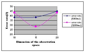
In the final set of MLP experiments, we have tried to optimize the length of the analysis
Classifier
Error rate (%)
window. In Fig. 10, error rates are shown for two window lengths: 640 ms and 1280 ms. The
Artificial Neural Network MLP
24 %
results show a better performance with the larger window. An error rate of 27% was
SVM Polynomial Kernel
17 %
reached.
SVM Radial Basis Kernel
16.7 %
In the last experiment with MLP classifier, the non analytic grid is used. The other
SVM Hyperbolic Tangent Kernel
20 %
parameters were fixed to what is empirically found using the spherical grid. The error rate
Table 1. Error rates obtained with SVM classifiers compared to MLP.
decreased to 24%. This shows that the choice of the grid is critical.
In order to quantify the ability of the system to distinguish between “action” and “no
action” events and between “left action” and “right action” events, experiments with a two
classes-classification have been conducted. The results shown in Table 2 demonstrate that it
is much easier to distinguish between “action” and “no action” classes than to determine
which action has been thought. The Radial basis Kernel seems to provide the best results.
These results outperform the best result obtained in (Sajda 2003), i.e. 24%.
Error rate (%)
Classifier
action/no action