UNIT – II
Lesson IV Production Analysis
At the end of reading of this chapter the reader will be able to understand that production is a function of land, labour, capital and organisation. The mangers will have to procure the right level of these factors based on factors like diminishing marginal utility economies of large scale operations, law of return, scales etc., with a view of maximizing the output with minimum cost so as to earn larger profit to the firm/industry.
Lesson Outline:
Introduction:
Production is an important economic activity which satisfies the wants and needs of the people. Production function brings out the relationship between inputs used and the resulting output. A firm is an entity that combines and processes resources in order to produce output that will satisfy the consumer’s needs. The firm has to decide as to how much to produce and how much input factors (labour and capital) to employ to produce efficiently. This chapter helps to understand the set of conditions for efficient production of an organization.
Factors of production include resource inputs used to produce goods and services. Economist categorise input factors into four major categories such as land, labour, capital and organization.
Land: Land is heterogeneous in nature. The supply of land is fixed and it is a permanent factor of production but it is productive only with the application of capital and labour.
Labour: The supply of labour is inelastic in nature but it differs in productivity and efficiency and it can be improved.
Capital: is a man made factor and is mobile but the supply is elastic.
Organization: the organization plans, , supervises, organizes and controls the business activity and also takes risks.
Production function indicates the maximum amount of commodity ‘X’ to be produced from various combinations of input factors. It decides on the maximum output to be produced from a given level of input, and how much minimum input can be used to get the desired level of output. The production function assumes that the state of technology is fixed. If there is a change in technology then there would be change in production function.
Q = f (Land, Labour, Capital, Organization)
Q = f (L, L, C, O)
The production manager’s responsibility is that of identifying the right combination of inputs for the decided quantity of output. As a manager ,he has to know the price of the input factors and the budget allocation of the organization. The major objective of any business organization is maximizing the output with minimum cost. To achieve the maximum output the firm has to utilize the input factors efficiently. In the long run, without increasing the fixed factors it is not possible to achieve the goal. Therefore it is necessary to understand the relationship between the input and output in any production process in the short and long run.
Cobb Douglas Production Function:
This is a function that defines the maximum amount of output that can be produced with a given level of inputs. Let us assume that all input factors of production can be grouped into two categories such as labour (L) and capital (K).The general equilibrium for the production function is
Q = f (K, L)
There are various functional forms available to describe production. In general Cobb-Douglas production function (Quadratic equation) is widely used

Q = the maximum rate of output for a given rate of capital (K) and labour (L).
Short Run Production Function:
In the short run, some inputs (land, capital) are fixed in quantity. The output depends on how much of other variable inputs are used. For example if we change the variable input namely (labour) the production function shows how much output changes when more labour is used. In the short run producers are faced with the problem that some input factors are fixed. The firms can make the workers work for longer hours and also can buy more raw materials. In that case, labour and raw material are considered as variable input factors. But the number of machines and the size of the building are fixed. Therefore it has its own constraints in producing more goods.
In the long run all input factors are variable. The producer can appoint more workers, purchase more machines and use more raw materials. Initially output per worker will increase up to an extent. This is known as the Law of Diminishing Returns or the Law of Variable Proportion. To understand the law of diminishing returns it is essential to know the basic concepts of production.
Measures Of Productivity
Total production (TP): the maximum level of output that can be produced with a given amount of input.
Average Production (AP): output produced per unit of input AP = Q/L
Marginal Production (MP): the change in total output produced by the last unit of an input
Marginal production of labour =  Q / L (i.e. change in the quantity produced to a given change in the labour)
Marginal production of capital = Q / K (i.e. change in the quantity produced to a given change in the capital)
Production Function:
A production function, like any other function can be expressed and analysed by any one or more of the three tools namely table, graph and equation. The maximum amounts of output attainable from various alternative combinations of input factors are given in the table.
The production function expressed in tabular form is as follows.
Table - Production Schedule
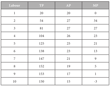
The firm has a set of fixed variables. As long with that it increases the labour force from 1 unit to 10 units. The increase in input factor leads to increase in the output up to an extent. After that it start declining. Marginal production increases in the initial period and then it starts declining and it become negative. The firm should stop increasing labour force if the marginal production is zero-that is the maximum output that can be derived with the available fixed factors. The 9th labour does not contribute to any output. In case the firm wants to increase the output beyond 153 units it has to improve its fixed variable. That means purchase of new machinery or building is essential. Therefore the firm understands that the maximum output is 153 units with the given set of input factors.
The graphical representations of the production function are as shown in the following graph.
Graph-Production Curves
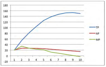
The graphical presentations of the values are shown in the graph. The ‘X” axis denotes the labour and the ‘Y’ axis indicates the total production (TP), average production (AP) and marginal production (MP). From the given table and graph we can understand all the three curves in the graph increased in the beginning and the marginal product (MP) first fell, then the average product (AP) finally total production (TP). The marginal production curve MP cuts the AP at its highest point. Total production TP falls when marginal production curve cuts the ‘X’ axis. The law of diminishing returns states that if increasing quantity of a variable input are combined with fixed, eventually the marginal product and then average product will decline.
When the production function is expressed as an equation it shall be as follows:
Q = f (Ld, L, K, M, T )
It can be expressed as Q = f1, f2, f3, f4, f5 > 0
Where,
Q = Output in physical units of good X
Ld = Land units employed in the production of Q
L = Labour units employed in the production of Q
K = Capital units employed in the production of Q
M = Managerial Units employed in the production of Q
T = Technology employed in the production of Q
f = Unspecified function
fi = Partial derivative of Q with respect to ith input.
This equation assumes that output is an increasing function of all inputs.
In the combination of input factors when one particular factor is increased continuously without changing other factors the output will increase in a diminishing manner. Let us assume that a person preparing for an examination continuously prepares without any break. The output or the understanding and the coverage of the syllabus will be more in the beginning rather than in the later stages. There is a limit to the extent to which one factor of production can be substituted for another. The total production increases up to an extent and it gets saturated or there won’t be any change in the output due to the addition of the input factor and further it leads to negative impact on the output. That means the marginal production declines up to an extent and it reaches zero and becomes negative. The point at which the MP becomes zero is the maximum output of the firm with the given set of input factors. This law is applicable in all human activities and business activities.
For example with two sewing machines and two tailors, a firm can produce a maximum of 14 pairs of curtains per day. The machines are used only from 9 AM to 5 PM and the machines lie idle from 5 pm onwards. Therefore the firm appoints 2 more tailors for the second shift and the production goes up to 28 units. Then adding two more labour to assist these people will increase the output to 30 units. When the firm appoints two more people, then there won’t be any change in their production because their Marginal productivity is zero. There is no addition in the total production. That means there is no use of appointing two more tailors. Therefore, there is a limit for output from a fixed input factors but in the long run purchase of one more sewing machine alone will help the firm to increase the production more than 30 units.
The Law Of Returns To Scale
In the long run the fixed inputs like machinery, building and other factors will change along with the variable factors like labour, raw material etc. With the equal percentage of increase in input factors various combinations of returns occur in an organization.
Returns to scale: the change in percentage output resulting from a percentage change in all the factors of production. They are increasing, constant and diminishing returns to scale.
Increasing returns to scale may arise: if the output of a firm increases more than in proportionate to an increase in all inputs. For example the input factors are increased by 50% but the output has doubled (100%).
Constant returns to scale: when all inputs are increased by a certain percentage the output increases by the same percentage. For example input factors are increased by 50% then the output has also increased by 50 percentages. Let us assume that a laptop consists of 50 components we call it as a set. In case the firm purchases 100 sets they can assemble 100 laptops but it is not possible to produce more than 100 units.
Diminishing returns to scale: when output increases in a smaller proportion than the increase in inputs it is known as diminishing return to scale. For example 50% increment in input factors lead to only 20% increment in the output.
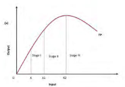
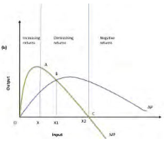
From the graph given below we can see the total production (TP) curve and the marginal production curve (MP) and average production curve (AP). It is classified into three stages; let us understand the stages in terms of returns to scale.
Stage I: The total production increased at an increasing rate. We refer to this as increasing stage where the total product, marginal product and average production are increasing.
Stage II: The total production continues to increase but at a diminishing rate until it reaches the next stage. Marginal product, average product are declining but are positive. The total production is at the maximum level at the end of the second stage with a zero marginal product.
Stage III: In this third stage total production declines and marginal product becomes negative. And the average production also started decline. Which implies that the change in input factors there is a decline in the over all production along with the average and marginal.
In economics, the production function with one variable input is illustrated with the well known law of variable proportions. (below graph) it shows the input-output relationship or production function with one factor variable while other factors of production are kept constant. To understand a production function with two variable inputs, it is necessary know the concept iso-quant or iso-product curve.
ISO-Quants
To understand the production function with two variable inputs, iso-quant curve is used. These curves show the various combinations of two variable inputs resulting in the same level of output. The shape of an Iso-quant reflects the ease with which a producer can substitute among inputs while maintaining the same level of output. From the graph we can understand that the iso-quant curve indicates various combinations of capital and labour usage to produce 100 units of motor pumps. The points a, b or any point in the curve indicates the same quantum of production. If the production increases to 200 or 300 units definitely the input usage will also increase therefore the new iso-quant curve for 200 units (Q1) is shifted upwards. Various iso-quant curves presented in a graph is called as iso-quant map.
Iso-cost: different combination of inputs that can be purchased at a given expenditure level.
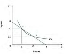
The above graph explains clearly that the iso quant curve for 100 units of motor consists of ‘n’ number of input combinations to produce the same quantity. For example at ‘a’ to produce 100 units of motors the firm uses OC amount of capital and OL amount of labour ie., more capital and less labour force. At ’b’ OC1 amount of capital and OL1 labour force is used to produce the same that means more labour and less capital.
Optimal input combination: The points of tangency between iso quant and iso cost curves depict optimal input combination at different activity levels.
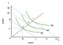
Expansion path: Optimal input combinations as the scale of production expand. From the graph it is clear that the optimum combination is selected based on the tangency point of iso cost (budget line) and iso-quant ie., a, b respectively. The point ‘a’ indicates that to produce 100 units of motor the best combination of capital and labour are OC and OM which is within the budget. Over a period of time a firm will face various optimum levels if we connect all points we derive expansion path of a firm.
Managerial Uses Of Production Function:
Production functions are logical and useful. Production analysis can be used as aids in decision making because they can give guidance to obtain the maximum output from a given set of inputs and how to obtain a given output from the minimum aggregation of inputs. The complex production functions with large numbers of inputs and outputs are analyzed with the help of computer based programmes.
Review Questions
*****