Lesson V Cost Analysis
At the end of reading this chapter the reader will be able to understand the concepts like fixed cost, variable cost, average cost, and marginal cost. The concept of the marginal costing is the contribution of the 20th century. The concept like break even analysis, cost volume profit analysis are the important tools used to take various managerial decisions. The concept like average revenue decides the level of output to earn profit. At the same time the concept like marginal cost is the tool available in the hands of the producers to decide that level of output where MC = AR i.e., the equilibrium position of the suppliers and consumers.
Lesson Outline:
Introduction:
A production function tells us how much output a firm can produce with its existing plant and equipment. The level of output depends on prices and costs. The most desirable rate of output is the one that maximizes total profit that is the difference between total revenue and total cost.
Entrepreneurs pay for the input factors-Wages for labour, price for raw material, rent for building hired, interest for borrowed money. All these costs are included in the cost of production. The economist’s concept of cost of production is different from accounting.
This chapter helps us to understand the basic cost concepts and the cost output relationship in the short and long runs. Having looked at input factors in the previous chapter it is now possible to see how the law of diminishing returns affect short run costs.
The cost of production of goods and services depends on various input factors used by the organization and it differs from firm to firm. The major cost determinants are:
There are various classifications of costs based on the nature and the purpose of calculation. But in economics and for accounting purpose the following are the important cost concepts.
Actual cost/ Outlay cost/ Absolute cost / Accounting cost: The cost or expenditure which a firm incurs for producing or acquiring a good or service. (Eg. Raw material cost)
Opportunity cost: The revenue which could have been earned by employing that good or service in some other alternative uses. (Eg. A land owned by the firm does not pay rent. Thus a rent is an income forgone by not letting it out)
Sunk cost: Are retrospective (past) costs that have already been incurred and cannot be recovered.
Historical cost: The price paid for a plant originally at the time of purchase.
Replacement cost: The price that would have to be paid currently for acquiring the same plant.
Incremental cost: Is the addition to costs resulting from a change in the nature of level of business activity. Change in cost caused by a given managerial decision.
Explicit cost: Cost actually paid by the firm. If the factors of production are hired or rented then it is an explicit cost.
Implicit cost: If the factors of production are owned by a firm then its cost is implicit cost.
Book cost: Costs which do not involve any cash payments but a provision is made in the books of accounts in order to include them in the profit and loss account to take tax advantages.
Social cost: Total cost incurred by the society on account of production of a good or service.
Transaction cost: The cost associated with the exchange of goods and services.
Controllable cost: Costs which can be controllable by the executives are called as controllable cost.
Shut down cost: Cost incurred if the firm temporarily stops its operation. These can be saved by continuing business.
Economic costs are related to future. They play a vital role in business decisions as the costs considered in decision - making are usually future costs. They are similar in nature to that of incremental, imputed explicit and opportunity costs.
Determinants Of Short –Run Cost
Fixed cost: Some inputs are used over a period of time for producing more than one batch of goods. The costs incurred in these are called fixed cost. For example amount spent on purchase of equipment, machinery, land and building.
Variable cost: When output has increased the firm spends more on these items. For example the money spent on labour wages, raw material and electricity usage. Variable costs vary according to the output. In the long run all costs become variable.
Total cost: The market value of all resources used to produce a good or service.
Total Fixed cost: Cost of production remains constant whatever the level of output.
Total Variable cost: Cost of production varies with output.
Average cost: Total cost divided by the level of output.
Average variable cost: Variable cost divided by the level of output.
Average fixed cost: Total fixed cost divided by the level of output.
Marginal cost: Cost of producing an extra unit of output.
Fixed cost curve is a horizontal line which is parallel to the ‘X’ axis. This cost is constant with respect to output in the short run. Fixed cost does not change with output. It must be paid even if ‘0’ units of output are produced. For example: if you have purchased a building for the business you have invested capital on building even if there is no production.
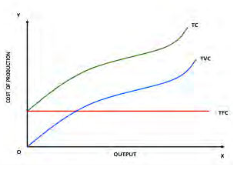
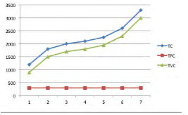
Total fixed cost (TFC) consists of various costs incurred on the building, machinery, land, etc.. For example if you have spent Rs. 2 Lakhs and bought machinery and building which is used to produce more than one batch of commodity, then the same cost of Rs. 2 Lakhs is fixed cost for all batches. The total variable costs vary according to the output. Whenever the output increases the firm has to buy more raw materials, use more electricity, labour and other sources therefore the TVC curve is upward sloping. The total cost consists of fixed (TFC) and variable costs (TVC). The TFC of Rs. 2 Lakhs is included with the variable cost throughout the production schedule so the total cost (TC) is above the TVC line.
Graph – Total Cost Curves
Graph – Average Cost Curves
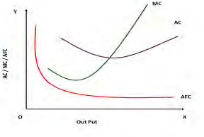
The above set of graphs indicates clearly that the average variable cost curve looks like a boat. Average fixed cost curve declines as output increases and it is a hyperbola to the origin. The Marginal cost curve slopes like a tick mark which declines up to an extent then it starts increasing along with the output. Let us see and understand the nature of each and every curve with an example. The table and graphs shown below indicates the total costs curves and average cost curves at various output level.
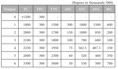
Table - Cost Schedule
Graph – Average Cost Curves
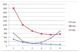
Graph – Total Cost Curves
From the above table and set of graphs we can understand that capital is the fixed factor of production and the total fixed cost will be the same Rs. 300,000. The total variable cost will increase as more and more goods are produced. So the total variable cost TVC of producing 1 unit is Rs.1500 000, for 2 units 1700 000 and so on.
Total cost = TFC + TVC for 1 unit TC = 300 + 1500 = 1800.
The marginal cost of producing an extra unit is calculated based on the difference in total cost.
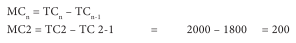
MC for 5th unit = TC of 5th unit minus TC of 4th unit, in our example 2600 – 2250 = 350.
AVC also is calculated in the same manner TVC / output = 2600 / 5 = 460 AFC = TFC / output = 300 / 5 = 60.
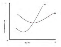
Relationship Between Marginal Cost And Average Cost Curve:
The marginal cost and average cost curves are U shaped because of law of diminishing returns. The marginal cost curve cuts the average cost curve and average variable cost curves at their lowest point. Marginal cost curve cuts the average variable cost from below. The AC curve is above the MC curve when AC is falling. The AC curve is below the MC when AC is increasing. The intersecting point indicates that AC=MC and that is the minimum average cost with an optimum output. (No more output can be produced at this average cost without increasing the fixed cost of production)
Graph – Relationship Between Average Cost And Marginal Cost
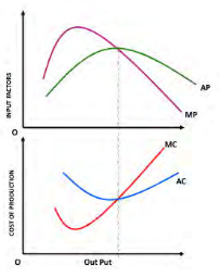
The MC and AC curves are mirror image of the MP and AP curves. It is presented in the graph below.
All organizations aim for maximum output with minimum cost. To achieve this goal they like to derive the point where optimum output can be produced with the given amount of input factors and with a minimum average cost. In the graph the MP=AP at maximum average production. On the other hand MC = AC at minimum average variable cost. Therefore this is the optimum output to be produced to achieve their managerial goals.
Graph – Optimum Cost And Output
The above set of cost curves explain the cost output relationship in the short period but in the long run there is no fixed cost because all costs vary over a period of time. Therefore in the long run the firm will have only average cost curve that is called as long run average cost curve (LAC). Let us see how the average cost curve is derived in the long run. This LAC also slopes like the short period average cost curve (U shaped) provided the law of diminishing returns prevails. In case the returns to scale are increasing or constant then the LAC curve will have a different slope. It will be a horizontal line, which is parallel to the ‘X’ axis.
Cost Output Relationship In The Long Run
In the long run costs fall as output increases due to economies of scale, consequently the average cost AC of production falls. Some firms experience diseconomies of scale if the average cost begins to increase. This fall and rise derives a U shaped or boat shaped average cost curve in the long run which is denoted as LAC. The minimum point of the curve is said to be the optimum output in the long run. It is explained graphically in the chart given below.
Graph – Long Run Average Cost Curve
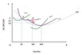
In the long run all factors are variable and the average cost may fall or increase to A, B respectively but all these costs are above the long run cost average cost. LAC is the lower envelope of all the short run average cost curves because it contains them all. At point ‘E’ the SAC1 and SMC1 intersects each other, in case the organization increases its output from OM to OM1 they have to spend OC1 amount. In case the organization purchases one more machine (increase in fixed cost) then they will get a new set of cost curves SAC2, and SMC2. But the new average cost curve reduces the cost of production from OC1 to OC2.That means they can save the difference of C1C2 which is nothing but AB. Therefore in the long run due to business expansion a firm can reduce their cost of production. During their business life they will meet many combinations of optimum production and minimum cost in different short periods. In the long run due to law of diminishing returns the long run average cost curve LAC also slopes like boat shape.
Economies Of Scale
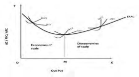
Economies of scale exist when long run average costs decline as output is increased. Diseconomies of scale exist when long run average cost rises as output is increased. It is graphically presented in the following graph. The economies of scale occur because of (i) technical economies: the change in production process due to technology adoption. (ii) Managerial economies (iii) purchasing economies, (iv) marketing economies and (v) financial economies.
Economies of scale means a fall in average cost of production due to growth in the size of the industry within which a firm operates.
Diseconomies Of Scale:
Arises due to managerial problems. If the size of the business becomes too large, then it becomes difficult for management to control the organizational activities therefore diseconomies of scale arise.
Graph – Economies of Scale and Diseconomies of scale
Factors Causing Economies Of Scale:
There are various factors influencing the economies of scale of an organization. They are generally classified in to two categories as Internal factors and External factors.
Internal Factors:
External Factors:
Factors Causing Diseconomies Of Scale:
Constant Returns To Scale:
In the long run if the returns to scale are constant then the average cost of production will be the same. For example : Ananda Vikatan magazine, started 100 years ago and it was sold in the market for 25 paise but now it is still sold at a nominal cost of Rs.15. The price increased because raw material cost and printing and labour costs have also increased but in the long run the price of the commodity has not increased much.
The constant returns to scale curve is graphically presented below which indicates that the LRAC is not a boat shaped curve.
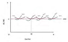
From the above graph it is clear that in the long run it is possible to derive a LRAC as a straight line with constant returns to scale.
Economies of scope: producing variety to get cost advantage. In retail business it is commonly used. Product diversification within the same scale of plant will help them to achieve success.
Lessons For Managers:
Review Questions:
Break Even Analysis
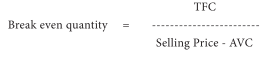
Break even analysis helps to identify the level of output and sales volume at which the firm ‘breaks even’. It means the revenues are sufficient to cover all costs of production. Various managerial decisions of firms are taken by the managers based on the break-even point.
It is a study of cost, revenues and sales of a firm and finding out the volume of sales where the firm’s costs and revenues will be equal. There is no profit and no loss. The total revenue is equal to the total cost of production. The amount of money which the firm receives by the sale of its output in the market is known as revenue.
Graph – Break Even Point
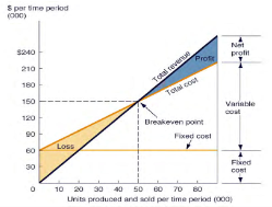
The above graph shows the break-even point of an organization. The total revenue curve (TR) and total cost curve (TC) is given. When they produce 50 units the total cost and total revenue are equal that is $ 150’000 which is at the intersecting point of the curves. Break even point always denotes the quantity produced or sold to equalize the revenue and cost.
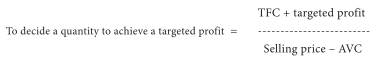
When the firm produces less than 50 units the revenue earned is less than the cost of production (TR<TC) therefore in the initial period the firm incurs loss which is shown in the graph. Through selling more than 50 units the revenue increases more than the cost of production therefore the difference increases and provides profit to the organization (TR>TC). It can be calculated with the help of the following formula.
Managerial Uses Of Break-Even Analysis:
We can conclude that the break – even analysis is a useful tool for decision making at various levels of a business firm in the short and long run. Therefore it is an essential tool to be used by the Managers.
Review Questions:
*****