Neural Network
In general we call it “Artificial Neural Network (ANN)” as it performs similar to human brain neurons (simpler version of it). The network is made of Input nodes, output nodes which are connected through hidden nodes and links (they carry weightage). Like human brain trains the neuron by various instances/situations and designs its reaction towards it, the network learns the input and its reaction in output, through algorithm and using machine learning.
There are single layer feed forward, multilayer feed forward and recurrent layer network architecture exists. We will see the single layer feed forward in this case. Single layer of nodes which uses inputs to learn towards outputs are single layer feed forward architecture.
In Neural Network we need the network to learn and develop the patters and reduce the overall network error. Then we will validate the network using a proportion of data to check the accuracy. If the learning and validation total mean squared error is less (Back propagation method-by forward and backward pass the weights of the link are adjusted, recursively) then the network is stable.
In general we are expected to use continuous variable, however discrete data is also supported with the new tools. Artificial Neural Networks is a black box technique where the inputs are used to determine the outputs but with hidden nodes, which can’t be explained by mathematical relationships/formulas. This is a non-linear method which tends to give better results than other linear models.
Neural Networks - Steps
We are going to explain neural networks using JMP tool from SAS. As we discussed in regression, this tool is versatile and provides detailed statistics.
Collect the data and check for any high variations and see the accuracy of it.
Use the Analyze->modelling->Neural from the tool and provide X and Y details. In JMP we can give discrete data also without any problem.
In the next step we are expected to specify the number of hidden nodes we want to have. Considering the normal version of JMP is going to allow single layer of nodes, we may specify as a rule of thumb (count of X’s * 2).
We need to specify the method by which the data will be validated, here if we have enough data (Thumb Rule: if data count> count of X’s * 20) then we can go ahead with ‘Holdback’ method, where certain percentage of data is kept only for validation of the network, else we can use Kfold and give to give number of folds (each fold will be used for validation also). In Holdback method keep 0.2 (20%) for validation.
We get the results with Generalized R2, and here if the value is nearer to 1 means, the network is contributing to prediction (the variables are able to explain well of the output, using this neural network). We have to check the validation R2 also to check how good the results are. Only when the training and validation results are nearly the same, the network is stable and we can use for prediction. In fact the validation result in a way gives the accuracy of the model and their error rate is critical to be observed.
The Root Mean Squared Error to be minimum. Typically you can compare the fit model option given in JMP which best fits the linear models and compare their R2 value with Neural Networks outcome.
The best part of JMP is its having interactive profiler, which provides information of X’s value and Y’s outcome in a graphical manner. We can interactively move the values of X’s and we can see change in ‘Y’ and also change in other X’s reaction for that point of combination.
With this profiler there is sensitivity indicator (triangle based) and desirability indicator. This acts as optimizer, where we can set the value of “Y” we want to have with Specification limits/graphical targets and for which the X’s range we will be able to get with this. There are maximization, minimization and target values for Y.
Simulation is available as part of profiler itself and we can fix values of X’s (with variation) and using monte carlo simulation technique the tool provides simulation results, which will be helpful to understand the uncertainties.
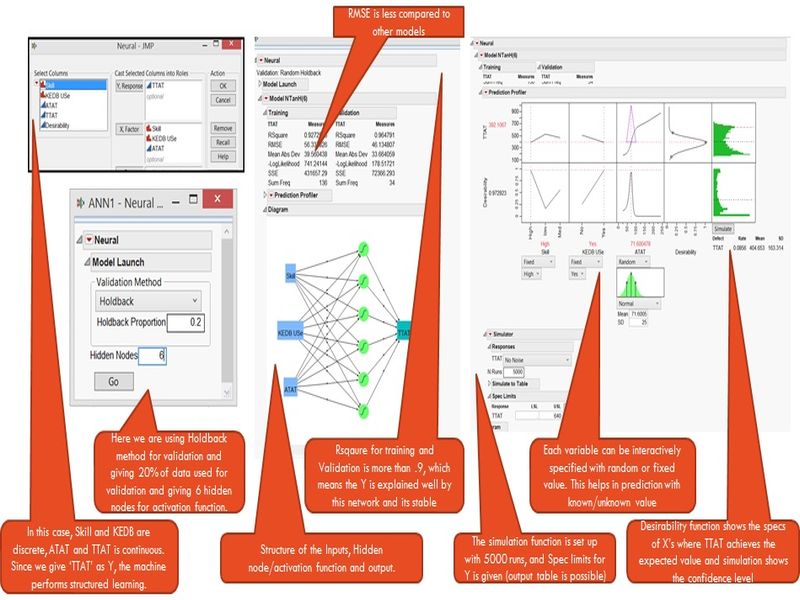
Neural Networks - Sample
Assume a case in which we have a goal of Total Turn-Around-Time (TTAT) (Less than 8hrs is target). The variables which is having influence are Skill (H, M, L), KEDB (Known Error Database) Use (Yes, No) and ATAT (Analyse Turn-Around-Time), How do we go with Neural Networks based on previous steps. (Around 170 data points collected from project is used)
Neural Network Tools
Matlab has neural network toolbox and which seems to be user friendly and has many options and logical steps to understand and improve the modelling. What we are not sure is the simulation and optimization capabilities. The best part is they give relevant scripts which can be modified or run along with existing tools.
JMP has limitations when it comes to Neural Network as only single layer of hidden network can be created and options to modify learning algorithm are limited. However JMP Pro has relevant features with many options to fit our need of customization.
Minitab at this moment doesn’t have neural networks in it. However SPSS tool contains neural network with multilayer hidden nodes formation capabilities.
Nuclass 7.1 is a free tool (professional version has cost) which is specialized in Neural Network. There are many options available for us to customize the model. However it won’t be as easy like JMP or SPSS.
PEERForecaster and Alyuda Forecaster are excel based neural network forecasting tools. They are easy to use to build the model, however the simulation and optimization with controllable variable is question mark with these tools.