Reliability Modelling
Reliability is an attribute of software product which implies the probability to perform at expected level without any failure. The longer the software works without failure, the better the reliability. Reliability modelling is used in software in different conditions like defect prediction based on phase-wise defect arrival or testing defect arrival pattern, warranty defect analysis, forecasting the reliability, etc. Reliability is measured in a scale of 0 to 1 and 1 is more reliable.
There is time dependent reliability, where time is an important measure as the defect occurs with time, wear out, etc. There is also non-time dependent reliability; in this case though time is a measure which communicates the defect, the defect doesn’t happen just by time but by executing faulty programs/codes in a span of time. This concept is used in software industry for MTTR (Mean Time To Repair), Incident Arrival Rate, etc.
Software reliability models normally designed with the distribution curve which depicts the shape where defect identification/arrival with time reduces from peak towards a low and flatter trajectory. The shape of the curve is the best fit model and most commonly we use weibull, logistic, lognormal, small extreme value probability distributions to fit. In software it’s also possible that every phase or period might be having different probability distributions.
Typically the defect data can be used in terms of count of defects in a period (ex: 20 / 40 / 55 in a day) or defect arrival time (ex: 25, 45, 60 minutes difference in which each defect entered). The PDF (Probability Distribution Function) and CDF (Cumulative Distribution Function) are important measures to understand the pattern of defects and to predict the probability of defects in a period/time, etc.
Reliability Modelling- Steps
We will work on Reliability again using JMP, which is pretty for this type of modelling. We will apply reliability to see the defects arrival in maintenance engagement, where the application design complexity and skill of people who are maintaining the software varies. Remember when we develop a model, we are talking about something controllable is there, if not these models are only time dependent ones and can only help in prediction but not in controlling.
In reliability we call the influencers as Accelerator, which impacts the failure. We can use weights of defects or priority as frequency and for the data point for which we are not sure about time of failure, we use Censor. Right censor is for the value for which you know only the minimum time beyond which it failed and left censor is for maximum time within which it failed. If you know the exact value, then by default it’s uncensored. There are many variants within reliability modelling; here we are going to use only Fit life by X modelling.
Collect the data with defect arrival in time or defect count by in time. In this case we are going to use Life fit by X, so we can collect it by time between defects. Also update the applications complexity and team skill level along with each data entry.
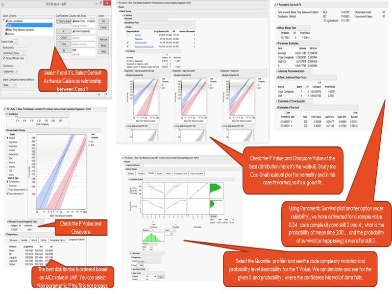
Select “Time to Event” as Y and select the accelerator (complexity measure) and use skill as separator.
There are different distributions which are categorized by the application complexity is available. Here we have to check the Wilcoxon Group Homogeneity Test for the P value (should be less than 0.05) and ChiSquare value (should be minimal).
To select the best fit distribution, look at the comparison criteria given in the tool, which shows -2logliklihood, AICc, BIC values. Here AICc (Corrected Akaike’s Information Criterion) should be minimal for the selected Distribution. BIC is Bayesian Information Criterion, which is stricter as it takes the sample size in to consideration. (In other tools, we might have Anderson Darling values, in that case select the one which has value less than or around 3 or the lowest)
In the particular best fit distribution, study the results for P-value, see the residual plot (Cox-Snell Residual P-plot) for their distribution.
Quantile Tab in this tool is used for extrapolation (ex: in Minitab, we can provide new parameters in a column and predict the values using estimate option) and for predicting the probability.
The variation of accelerator can be configured and probability is kept normally at 0.5 to see that 50% of chance or to be in the median and then the expected Mean time can be kept as LSL and/or USL accordingly. The simulation results will tell us the Mean and SD, with graphical results.
For Optimization on maintaining the Accelerator, we can use Set desirability function and can give a target for “Y” and can check the values.
Under Parametric survival option in JMP, we can check the probability of a defect arrival in a given time, using Application complexity and Skill level.
Reliability Modelling- Sample
Let’s consider the previous example where the complexity of applications are maintained at different level (controllable, assuming the code and design complexity is altered with preventive fixes and analysers) and that’s an accelerator for defect arrival time (Y) and skill of the team also plays a role (assuming the applications are running for quite some time and many fixes are made). In this case, we want to know the probability of having mean time arrival of defect/incident beyond 250 hrs.
Reliability Modelling- Tools
Minitab also has reliability modelling and can perform almost all types of modelling which other professional tools offer. For the people who are convenient with Minitab can use these options. However we have to remember that simulation and optimization is also a need for us in modelling in CMMI, so we may need to generate outputs and create ranges and simulate and optimize using Crystal ball (or any simulation tool).
Reliasoft - RGA is another tool with extensive features in reliability modelling. It’s comparatively user friendly tool. It’s a tool worth a try if reliability is our key concern.
R- though we don’t talk much about this free statistical package, it comes with loads of add on package for every need. We have never tried, may be because we are lazy and don’t want to go out of comfort from GUI abilities of other professional tools.
CASRE and SMERFS are free tools, which we have used in some context. However we never tried the Accelerators with these tools, so we are not sure are they having the option of life fit by X modelling. However for reliability forecasting and growth they are useful at no cost.
Matlab statistics tool box also contains reliability modelling features. SPSS reliability features are good enough to use for our needs in software Industry. However JMP is good from the point, that you only need one tool which gives modelling, simulation and optimization.
Process Modelling (Queuing System)
Queuing system is a one in which the entity arrival creates demand and it has to be served by limited resources assigned in the system. The system distributes its resources to handle various events in the system at any given point in time. The events are handled as discrete events in the system.
There are number of queuing systems can be created, however they are based on arrival of elements, servers utilization, wait time/time spent in the system flows (between servers and with the servers). Discrete events help the queuing model to capture the time stamps of different events and model their variation along with the queue system.
This model helps to understand the resource utilization of servers, bottlenecks in the system events, idle time, etc. Discrete Event Simulation with Queue is used in many places like banks, hospitals, airport queue management, manufacturing line, supply chain, etc.
In software Industry we can use in application maintenance incident/problem handling, Dedicated service teams /functions (ex: estimation team, technical review team, Procurement, etc), Standard change Request handling and in many contexts where the arrival rate and team size plays a role in delivering on time.
We also need to remember that in software context the element which comes in queue will be there in queue till its serviced and then it departs, unlike in a bank or hospital where a patient come late to the queue may not be serviced and they leave the queue.
Process Modelling -Steps
We will discuss the Queuing system modelling using the tool “Processmodel”.
Setting up flow:
It’s important to understand the actual flow of activities and resources in a system and then making a graphical flow and verifying it.
Once we are sure about the graphical representation, we have to provide the distribution of time, entity arrival pattern, resource capacity and assignment, input and output queue for each entity. These can be obtained by Time motion study of the system for the first time. The tool has Stat-fit, which will help to calculate the distributions.
Now the system contains entity arrival in a pattern with this by adding storage the entities will be retained till they get resolved. Resources can be given in shifts and by using get and free functions (we can code in a simple manner) and by defining scenarios (the controllable variables are given as scenario and mapped with values) their usage conditions can be modified to suit the actual conditions.