Regression
Regression is a process of estimating relationship among the dependant and independent variables and forming relevant explanation of for dependant variable with the conditional values of Independent Variables.
As a model its represented using Y=f(X) + error (unknown parameters)
Y – Dependent Variable, X –Independent Variables
Few assumptions related to regression,
Sample of data represents the population
The variables are random and their errors are also random
There is no multicollinearity (Correlation amongst independent variables)
We are working on here with multiple regression (with many X’s) and assuming linear regression (non linear regression models exist).
The X factors are either the measure of a sub process/process or it’s a factor which is influential to the data set/project /sample.
Regression models are often Static models with usage of historical data coming out from multiple usage of processes (many similar projects/activities)
Regression - Steps
Perform a logical analysis (ex: Brainstorming with fishbone) to understand the independent variables (X) given a dependent variable (Y).
Collect relevant data and plot scatter plots amongst X vs. Y and X1 vs. X2 and so on. This will help us to see if there is relationship (correlation) between X and Y, also to check on multicollinearity issues.
Perform subset study to understand the best subset which gives higher R2 value and less standard error.
Develop a model using relevant indications on characteristics of data with continuous and categorical data.
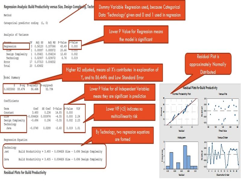
From the results study the R2 value (greater than 0.7 is good) which explains how much the Y is explained by X’s. The more the better.
Study the P values of Individual independent variables and it should be less than 0.05, which means there is significant relationship is there with Y.
Study the ANOVA Resulted P value to understand the model fit and it should be less than 0.05
VIF (Variance Inflation Factor) should be less than 5 (sample size less than 50) else less than 10, on violation of this multicollinearity possibility is high and X factors to be relooked.
Understand the residuals plot and it should be normally distributed, which means the prediction equation produces a line which is the best fit and gives variation on either side.
R2 alone doesn’t say a model is right fit in our context, as it indicates the Xs are pretty much relevant to the variation of Y, but it never says that all relevant X’s are part of the model or there is no outlier influence. Hence beyond that, we would recommend to validate the model.
Durbin Watson Statistic is used for checking Autocorrelation using the residuals, and its value ranges from 0 to 4. 0 indicates strong positive autocorrelation (previous data, impacts the successive time period data to increase) and 4 indicate strong negative autocorrelation (previous data, impacts the successive time period data to decrease) and 2 is no serial correlation.
Regression - Example
Assume a case where Build Productivity is Y, Size (X1), Design Complexity(X2) and Technology (X3 – Categorical data) are forming a model as the organization believes they are logically correlated. They collect data from 20 projects and followed the steps given in the earlier slide and formed a regression model and following are the results,
Validating model accuracy
Its important to ensure the model which we develop not only represents the system, but also has the ability to predict the outcomes with less residuals. In fact this is the part where we can actually understand whether the model meets the purpose.
To check the Accuracy we can use the commonly used method MAPE (Mean Absolute Percentage Error), which calculates the percentage error across observations between the actual value and predicted value.
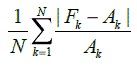
Where Ak is the actual value and Fk is the forecast value. An error value of less than 10% is acceptable. However if the values of forecasted observations are nearer to 0, then its better to avoid MAPE and instead use Symmetric Mean Absolute Percentage Error(SMAPE).
Interpolation & Extrapolation:
Regression models are developed using certain range of X values and the relationship holds true for within that region. Hence any data prediction, within the existing range of Xs (Interpolation) would mean we can rely on the results more. However the benefit of a model also relies on its ability to predict a situation which is not seen yet, in that cases, we expect the model to predict a range which it never encountered or the region in which the entire relationship or representation could significantly change between X’s and Y, which is extrapolation. To a smaller level extrapolation can be considered with uncertainty in mind, however larger variation of Xs, which is far away from the data used in developing the model, can be avoided as the uncertainty level increases.
Variants in Regression
Statistical relationship modelling is mainly selected based on the type of data which we have with us. The X factors and Y factors are continuous or discrete determines the technique to be used in developing the statistical model.
Data Type wise Regression:
Discrete X's and Continuous Y - ANOVA & MANOVA
Discrete X's and Discrete Y - Chi-Square & Logit
Continuous X's and Continuous Y - Correlation & Regression (simple/multiple/CART, etc)
Continuous X's and Discrete Y - Logistic Regression
Discrete and Continuous X's and Continuous Y - Dummy Variable Regression
Discrete and Continuous X's and Discrete Y - Ordinal Logit
By linearity, we can classify a regression as linear, quadratic, cubic or exponential. Based on type of distribution in the correlation space, we can use relevant regression model
Tools for Regression
Regression can be performed using Trendline functions of MS excel easily. In addition there are many free plug-ins available in the internet.
However from professional statistical tools point of view, Minitab 17 has easy features for users to quickly use and control. The tool has added profilers and optimizers which are useful for simulations and optimizations (earlier we were depending on external tools for simulation).
SAS JMP is another versatile tool with loads of features. If someone has used this tool for quite some time, they will be more addictive with its level of details and responsiveness. JMP had interactive profilers for quite a long period and can handle most of the calculations.
In addition, we have SPSS, Matlab tools which are also quite famous.
R is the open source statistical package which can be added with relevant add-ins to develop many models.
We would recommend considering the experience & competency level of users, licensing cost, complexity of modelling and ability to simulate & optimize in deciding the right tool.
Some organizations decide to develop their own tools, considering their existing source of data is in other formats; however we have seen such attempts rarely sustain and succeed. This is because, too much elapsed time, priority changes, complexity in algorithm development, limited usage, etc. Considering most of the tools support common formats, the organizations can consider to develop reports/data in these formats to feed in to proven tools / plugins.
Bayesian Belief Networks
A Bayesian Network is a construct in which the probabilistic relationships between variables are used to model and calculate the Joint Probability of Target.
The Network is based on Nodes and Arcs (Edges). Each variable represents a Node and their relationship with other Node is expressed using Arcs. If any given node is connected with a dependent on other variable, then it has parent node. Similarly if some other node depends on this node, then it has children node. Each node carries certain parameters (ex: Skill is a node, carries High, Medium, Low parameters) and they have probability of occurrence (Ex: High- 0.5, Medium -0.3, Low -0.2). When there is conditional independence (node has a parent) then its joint probability is calculated by considering the parent nodes (ex: Analyze Time being “Less than 4 hrs” or more, depends on Skill High/Med/Low, which is 6 different probability values).
The central idea of using this in modelling is based on the posterior probability can be calculated from the prior probability of a network, which has developed with the beliefs (learning). It’s based on Bayes Theorem.
Bayesian is used highly in medical field, speech recognition, fraud detection, etc
Constraints: The Method and supportive learning needs assistance and computational needs are also high. Hence its usage is minimal is IT Industry, however with relevant tools in place its more practical to use in IT.
Bayesian Belief Networks- Steps
We are going to discuss on BBN mainly using BayesiaLab tool, which has all the expected features to make comprehensive model and optimize the network and indicate the variables for optimization. We can discuss on other tools in upcoming slide.
In Bayesian, data of variables can be in discrete or continuous form; however they will be discredited using techniques like Kmeans/Equal Distance/Manual &other Methods.
Data has to be complete for all the observations in the data set for the variables, else the tool helps us to fill the missing data
Structure of the Network is important and it determines the relationship between variables, however it doesn’t often the cause and effect relationship instead a dependency. Domain experts along with process experts can define the structure (with relationship) manually.`
As an alternative, machine learning is available in the tool, where set of observations passed to the tool and using the learning options (structured and unstructured) the tool plots the possible relationships. The tool uses the MDL (Minimum Description Length) to identify the best possible structure. However we can logically modify the flow, by adding/deleting the Arcs (then, perform parameter estimation to updated the conditional probabilities)
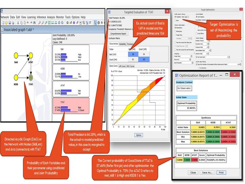
In order to ensure that the network is fit for prediction, we have to check the network performance. Normally this is performed using test data (separated from set of overall data) and use it to check the accuracy, otherwise the whole set is taken by tool to validate the model predicted values vs. actual value. This gives the accuracy of the network in prediction. Anything above 70% is good for prediction.
In other models we will perform simulation to see the uncertainty in achieving a target, but in probability model that step is not required, as the model directly gives probability of achieving.
In order to perform what if and understand the role each variable in maximizing the probability of target or mean improvement of target, we can do target optimization. This helps us to run number of trials within the boundaries of variation and see the best fit value of variables which gives high probability of achieving the target. Using these values we can compose the process and monitor the sub process statistically.
As we know some of the parameters with certainty, we can set hard evidence and calculate the probability. (Ex: Design complexity or skill is a known value, then they can be set as hard evidence and probability of productivity can be calculated.)
Arc Influence diagram will help us in understanding the sensitivity of variables in determining the Target.
Bayesian – Sample
Assume a case in which we have a goal of Total Turn-Around-Time (TTAT) with parameters Good (<=8hrs) and bad (>8hrs). The variables which is having influence are Skill, KEDB (Known Error Database) Use and ATAT (Analyse Turn-Around-Time) with Met (<=1.5 hrs) and Not met (>1.5hrs), How do we go with Bayesia modelling based on previous steps. (Each incident is captured with such data and around 348 incidents from a project is used)
Bayesian Tools
There are few tools few have worked on to get hands on experience. On selecting a tool for Bayesian modelling it’s important to consider that the tool has ability to machine learn, analyze and compare networks and validate the models. In addition the tool to have optimization capabilities.
GENIE is a tool from Pittsburgh University, which can help us learn the model from the data. The Joint probability is calculated in the tool and using hard evidence we can see the final change in probabilities. However the optimization parts (what if) is more of trial and error and not performed with specialized option.
We can use excels and develop the joint probabilities and verify with GENIE on the values and accuracy of the Network. The excel sheet can be used as input for simulation and optimization with any other tool (ex: Crystal ball) and what if can be performed. For sample sheets please connect with us in our mail id given in contact us.
In addition we have seen Bayes Server, which is also simpler in making the model; however the optimization part is not as easy we thought of.